This project consists of two parts: Part 1 aims to explore the data and optimize classifiers by fine-tuning hyperparameter. Part 2 continues with the fine-tuned models and optimize the classifiers via their decision thresholds.
Signals from MAGIC telescopes
This dataset was generated from a Monte Carlo program that simulates registration of high energy gamma particles detected by ground-based Major Atmospheric Gamma Imaging Cherenkov telescopes (MAGIC). When gamma rays (high energy photons) hit the Earth’s atmosphere, they interact with the atoms and molecules of the air to create a particle shower, producing blue flashes of light called Cherenkov radiation. This light is collected by the telescope’s mirror system and creates images of elongated ellipses. With this data, researchers can draw conclusions about the source of the gamma rays and discover new objects in our own galaxy and supermassive black holes outside of it.
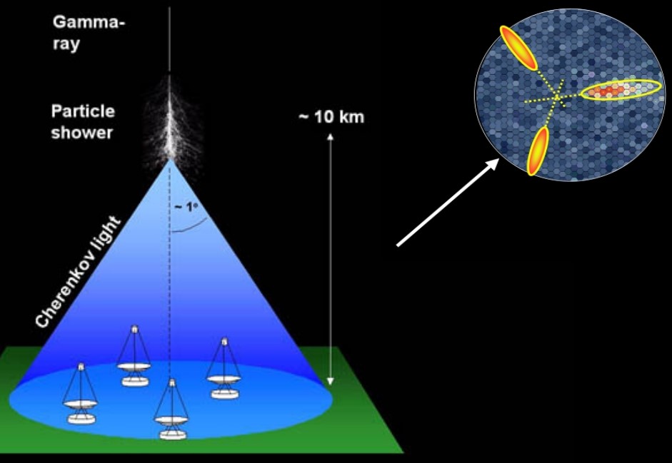
However, these events are also produced by hadron showers (atomic, not photonic) from cosmic rays. The goal is to utilize features of the ellipses to separate images of gamma rays (signal) from images of hadronic showers (background).
Python packages
import numpy as np
import pandas as pd
import seaborn as sns
import matplotlib.pyplot as plt
from sklearn.preprocessing import LabelEncoder, StandardScaler
from sklearn.model_selection import train_test_split, cross_val_score,  StratifiedKFold
from sklearn.model_selection import GridSearchCV, RandomizedSearchCV

from sklearn.decomposition import PCA

from sklearn.neighbors import KNeighborsClassifier
from sklearn.tree import DecisionTreeClassifier
from sklearn.ensemble import RandomForestClassifier
from sklearn.neural_network import MLPClassifier
from sklearn.metrics import accuracy_score, f1_score, make_scorer, confusion_matrix
Data exploration
This dataset contains 10 features derived from images of gamma ray (g) and hadronic (h) shower events.
| Feature | Description |
|---|---|
| fLength | Major axis of ellipse (mm) |
| fWidth | Minor axis of ellipse (mm) |
| fSize | 10-log of sum of content of all pixels |
| fConc | Ratio of sum of two highest pixels over fSize [ratio] |
| fConc1 | Ratio of highest pixel over fSize [ratio] |
| fAsym | Distance from highest pixel to center [mm] |
| fM3Long | 3rd root of third moment along major axis [mm] |
| fM3Trans | 3rd root of third moment along minor axis [mm] |
| fAlpha | Angle of major axis with vector to origin [deg] |
| fDist | Distance from origin to center of ellipse [mm] |
Read the csv data file.
Telescope = pd.read_csv('telescope.csv')
We see that all the features are floats and the class (g or h) is an object type.
Telescope.info()
<class 'pandas.core.frame.DataFrame'>
RangeIndex: 19020 entries, 0 to 19019
Data columns (total 11 columns):
 #   Column    Non-Null Count  Dtype
---  ------    --------------  -----
 0   fLength   19020 non-null  float64
 1   fWidth    19020 non-null  float64
 2   fSize     19020 non-null  float64
 3   fConc     19020 non-null  float64
 4   fConc1    19020 non-null  float64
 5   fAsym     19020 non-null  float64
 6   fM3Long   19020 non-null  float64
 7   fM3Trans  19020 non-null  float64
 8   fAlpha    19020 non-null  float64
 9   fDist     19020 non-null  float64
 10  class     19020 non-null  object
dtypes: float64(10), object(1)
There are no missing values, as expected from simulated data.
Telescope.isnull().sum()
fLength     0
fWidth      0
fSize       0
fConc       0
fConc1      0
fAsym       0
fM3Long     0
fM3Trans    0
fAlpha      0
fDist       0
class       0
dtype: int64
Using descrive, I can see that the features have very different ranges. This is not surprising, given that some features are ratios and others are 3rd root of values but it will be important to standardize them prior to classification.
Telescope.describe().loc[['count','mean','std','min','50%','max']]
            fLength        fWidth         fSize         fConc        fConc1  \
count  19020.000000  19020.000000  19020.000000  19020.000000  19020.000000
mean      53.250154     22.180966      2.825017      0.380327      0.214657
std       42.364855     18.346056      0.472599      0.182813      0.110511
min        4.283500      0.000000      1.941300      0.013100      0.000300
25%       24.336000     11.863800      2.477100      0.235800      0.128475
50%       37.147700     17.139900      2.739600      0.354150      0.196500
75%       70.122175     24.739475      3.101600      0.503700      0.285225
max      334.177000    256.382000      5.323300      0.893000      0.675200

              fAsym       fM3Long      fM3Trans        fAlpha         fDist
count  19020.000000  19020.000000  19020.000000  19020.000000  19020.000000
mean      -4.331745     10.545545      0.249726     27.645707    193.818026
std       59.206062     51.000118     20.827439     26.103621     74.731787
min     -457.916100   -331.780000   -205.894700      0.000000      1.282600
25%      -20.586550    -12.842775    -10.849375      5.547925    142.492250
50%        4.013050     15.314100      0.666200     17.679500    191.851450
75%       24.063700     35.837800     10.946425     45.883550    240.563825
max      575.240700    238.321000    179.851000     90.000000    495.561000
Count of events
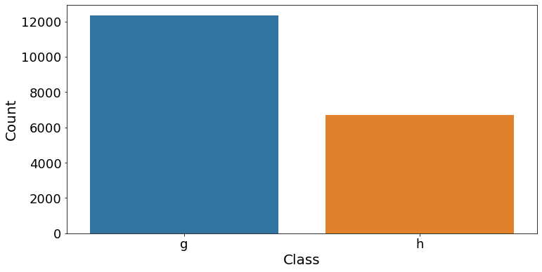
There is a bias towards a higher number of data points for gamma (12332) events than hadronic (6688) events. This suggests that we should use a machine learning score that is less sensitive to this type of bias, such as the F1 score.
# count of classes
Star['class'].value_counts()
# bar plot
fig, ax = plt.subplots(figsize=(12, 6))
sns.countplot(data=Star, x='class')
ax.set_xlabel('Class', fontsize=20)
ax.set_ylabel('Count', fontsize=20)
ax.tick_params(axis='both', which='major', labelsize=18)
plt.savefig('images/class.count.png')
plt.show()
g    12332
h     6688
Name: class, dtype: int64
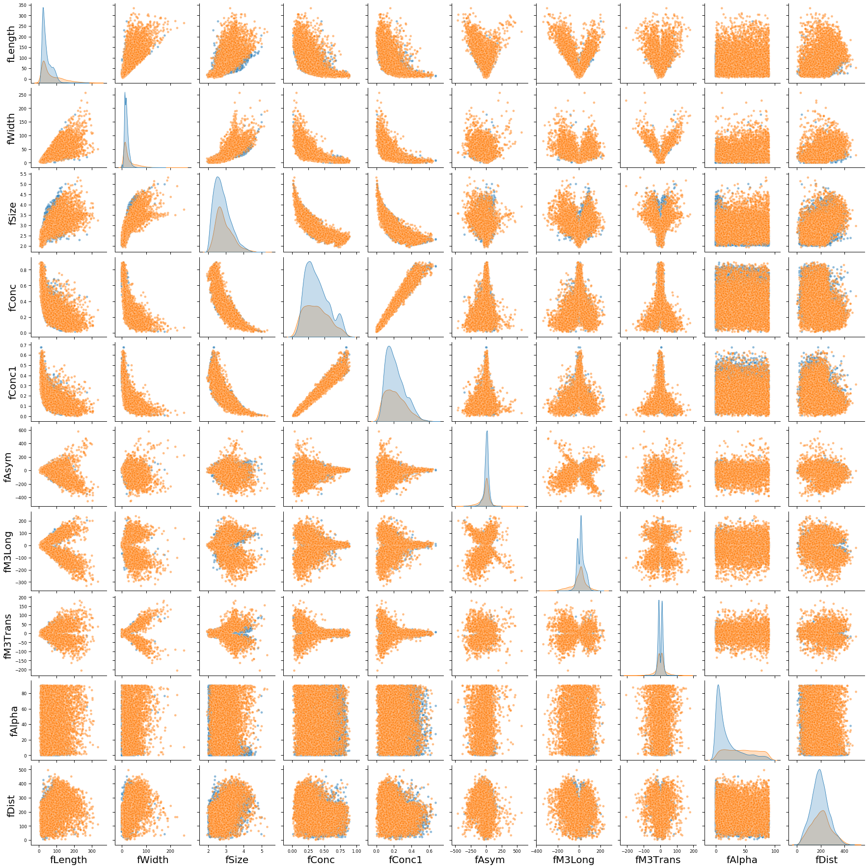
Pair plot of all features
sns.set_context("paper", rc={"axes.labelsize":20})
pp = sns.pairplot(Telescope, height = 2.5, hue='class', plot_kws={'alpha':0.5})
pp._legend.remove()
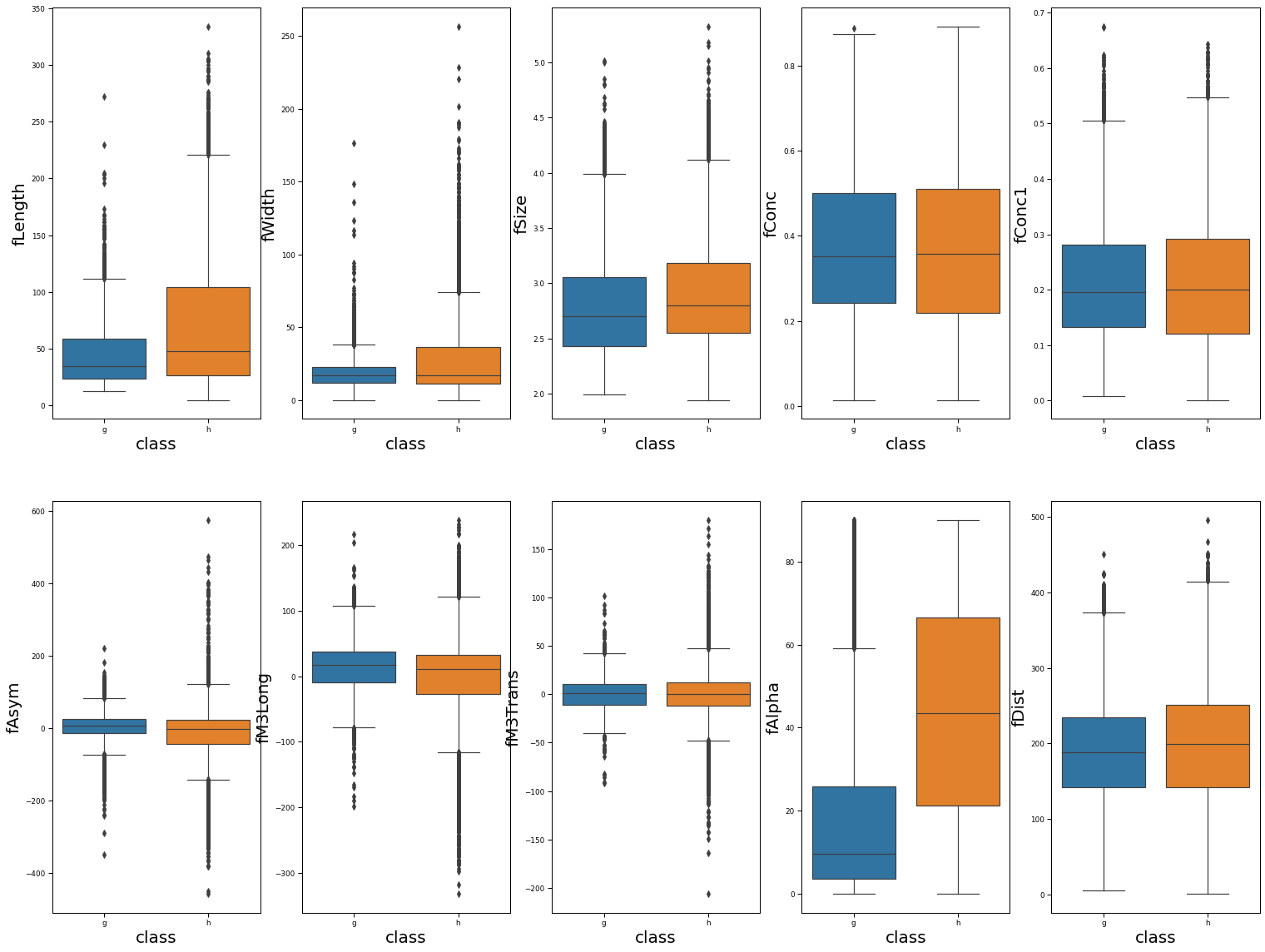
Boxplot of features
We observe that gamma and hadronic events have similar distributions for most individual features. The one exception is fAlpha, where the hadronic events tend to have larger values. Regardless, this indicates that any individual feature is unlikely to strongly differentiate gamma from hadronic events.
sns.set_context("paper", rc={"axes.labelsize":20})
fig, ax =plt.subplots(2, 5, figsize=(26,20))
sns.boxplot(x='class', y='fLength', data=Telescope, ax=ax[0,0])
sns.boxplot(x='class', y='fWidth', data=Telescope, ax=ax[0,1])
sns.boxplot(x='class', y='fSize', data=Telescope, ax=ax[0,2])
sns.boxplot(x='class', y='fConc', data=Telescope, ax=ax[0,3])
sns.boxplot(x='class', y='fConc1', data=Telescope, ax=ax[0,4])
sns.boxplot(x='class', y='fAsym', data=Telescope, ax=ax[1,0])
sns.boxplot(x='class', y='fM3Long', data=Telescope, ax=ax[1,1])
sns.boxplot(x='class', y='fM3Trans', data=Telescope, ax=ax[1,2])
sns.boxplot(x='class', y='fAlpha', data=Telescope, ax=ax[1,3])
sns.boxplot(x='class', y='fDist', data=Telescope, ax=ax[1,4])
fig.show()
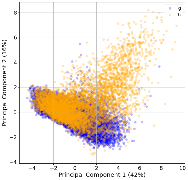
Principal components analysis
For classification problems, I typically perform a PCA to reduce dimensionality and see if the classes can be separated visually. Here, we see that the first and second principal components explain 42% and 16% of the variance.
# Get features and standardize using StandardScaler()
scaler = StandardScaler()
X = Telescope.drop('class', axis=1)
X_full_scaled = scaler.fit_transform(X)
# Perform PCA with 2 components
pca = PCA(n_components=2)
principalComponents = pca.fit_transform(X_full_scaled)
print(pca.explained_variance_ratio_)
[0.42239909 0.15751879]
When we plot this data, the gamma and hadronic events do not seem to cluster separately on these PCs. A lot of hadronic events cluster on the top-left side of the plot, but the majority clusters with the gamma events.
# Create dataframe for plotting
dfPC = pd.DataFrame(data = principalComponents, columns = ['principal component 1', 'principal component 2'])
dfFinal = pd.concat([dfPC, Telescope[['class']]], axis = 1)
# Plot data of PC axes
fig = plt.figure(figsize = (10,10))
ax = fig.add_subplot(1,1,1)
ax.set_xlabel('Principal Component 1', fontsize = 15)
ax.set_ylabel('Principal Component 2', fontsize = 15)
targets = ['g','h']
colors = ['blue','orange']
for target, color in zip(targets,colors):
    indicesToKeep = dfFinal['class'] == target
    ax.scatter(dfFinal.loc[indicesToKeep, 'principal component 1'],
               dfFinal.loc[indicesToKeep, 'principal component 2'],
               c=color, s=50, alpha=0.25)
ax.set_xlabel('Principal Component 1 (42%)', fontsize=20)
ax.set_ylabel('Principal Component 2 (16%)', fontsize=20)
ax.tick_params(axis='both', which='major', labelsize=18)
ax.legend(targets, prop={'size': 15})
ax.grid()
Data preprocessing
First I split the dataset in features (X) and classes (Y). I will utilize LabelEncoder to convert g and h into binary format in the class variable.
# Define X as features and Y as labels
X = Telescope.drop('class', axis=1)
Y = Telescope['class']
# Encode Y
le = LabelEncoder()
Y_encode = le.fit_transform(Y)
print(pd.crosstab(Y, Y_encode, rownames=['Original'], colnames=['Encode']))
Encode        0     1
Original
g         12332     0
h             0  6688
Now, split the data into the training and the test set using train_test_split. I will make the training set be 70% of the data and stratify by Y because the number of gamma and hadronic events are unbalanced.
# split to training and testing set, stratify by Y
X_train, X_test, Y_train, Y_test = train_test_split(X, Y_encode, test_size=0.30, stratify=Y)
Standardize each feature using StandardScaler because they vary a lot in their range (figure 3). Remember to only utilize the training set when fitting the scaler, that way no information from the test set will “leak” into the training set.
# Standardize X_train, then fit to X_test
scaler = StandardScaler()
scaler.fit(X_train)
X_train = scaler.transform(X_train)
X_test = scaler.transform(X_test)
Supervised machine learning
Here I explore using nearest neighbors, decision tree, random forest, and neural networks to classify the data. Since the number of gamma and hadron events are unbiased, I will focus on using the F1 score to determine the fit of the model. For each classifier, I will first perform optimization using GridSearchCV or RandomizedSearchCV to find the hyperparameters that maximize F1 on the training set. This will be followed by some exploratory analysis on the effects of select hyperparameters when performing cross-validation on the training set and ultimately when making predictions for the test set.
Below are wrapper functions for fine-tuning hyperparameters.
def grid_search_wrapper(model, parameters, cv, scoring):
    '''
    Perform grid search given model and parameters
    Outputs parameters and scores for best model
    '''
    # Perform grid search
    model_GS = GridSearchCV(model, parameters, cv=cv, scoring=scoring, verbose=1, n_jobs = 3)
    model_GS.fit(X_train, Y_train)
    print('Best parameters: ',model_GS.best_params_)
    print('Best score: ',model_GS.best_score_)
    # Test score
    Y_pred = model_GS.predict(X_test)
    print("Confusion matrix:\n", confusion_matrix(Y_test, Y_pred))
    print("F1:", f1_score(Y_test, Y_pred))
    print("Accuracy:", accuracy_score(Y_test, Y_pred))

def random_search_wrapper(model, parameters, cv, scoring, n_iter):
    '''
    Perform randomized search given model and parameters
    Outputs parameters and scores for best model
    '''
    # Perform grid search
    model_GS = RandomizedSearchCV(model, parameters, cv=cv, scoring=scoring, n_iter=n_iter, verbose=1, n_jobs = 3)
    model_GS.fit(X_train, Y_train)
    print('Best parameters: ',model_GS.best_params_)
    print('Best score: ',model_GS.best_score_)
    # Test score
    Y_pred = model_GS.predict(X_test)
    print("Confusion matrix:\n", confusion_matrix(Y_test, Y_pred))
    print("F1:", f1_score(Y_test, Y_pred))
    print("Accuracy:", accuracy_score(Y_test, Y_pred))
Nearest neighbors classifier
Hyperparameter tuning
Fine-tune weights, n_neighbors, and p. Utilize StratifiedKFold for cross-validation with 5 folds. Perform grid search on 160 models and 800 fits after accounting for cross-validation.
# Define model and parameters
model = KNeighborsClassifier()
cv = StratifiedKFold(n_splits=5)
parameters = {'weights':['uniform','distance'],
              'n_neighbors':[x for x in range(1, 41)],
              'p':[1,2]}
scoring = make_scorer(f1_score)
# Grid search
grid_search_wrapper(model, parameters, cv, scoring)
The best model has a training F1 of 0.736, and a test F1 of 0.743.
Best parameters:  {'n_neighbors': 5, 'p': 1, 'weights': 'distance'}
Best score:  0.7361074720702369
Confusion matrix:
 [[3520  180]
 [ 714 1292]]
F1: 0.7429557216791258
Accuracy: 0.843322818086225
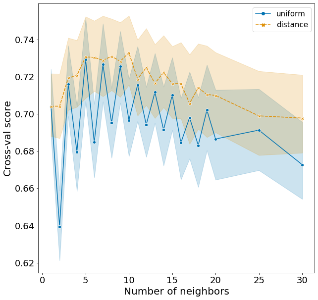
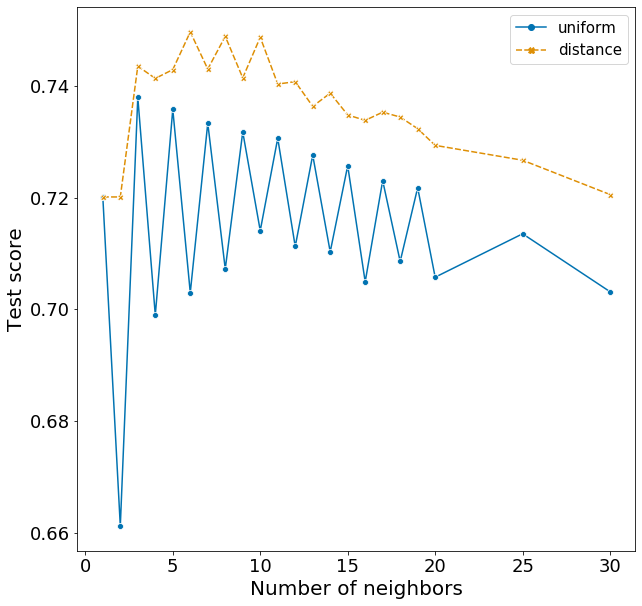
Explore hyperparameters
Here I explore the effects of weights and n_neighbors on F1, fixing the other parameters according to the best model from above.
# Parameters
p = 1
list_weights = ['uniform','distance']
list_n_neighbors = [x for x in range(1, 21)]+[25,30]
n_splits, scoring = 10, make_scorer(f1_score)

# Loop through all parameter combinations
results_cv = pd.DataFrame(columns=['weights','n_neighbors','CV_score'])
results_smy = pd.DataFrame(columns=['weights','n_neighbors','CV_mean_score','CV_std_score','Test_score'])
for weights in list_weights:
    for n_neighbors in list_n_neighbors:
        # define model and cv
        model = KNeighborsClassifier(p=p, weights=weights, n_neighbors=n_neighbors)
        cv = StratifiedKFold(n_splits=n_splits)
        # Cross-validation results
        n_scores = cross_val_score(model, X_test, Y_test, cv=cv, scoring=scoring, n_jobs = 3)
        CV_mean_score, CV_std_score = np.mean(n_scores), np.mean(n_scores)
        # Test set results
        model = model.fit(X_train, Y_train)
        Y_pred = model.predict(X_test)
        Test_score = f1_score(Y_test, Y_pred)
        # record all cv data
        for CV_score in n_scores:
            results_cv.loc[len(results_cv)] = [weights, n_neighbors, CV_score]
        # record summary data
        results_smy.loc[len(results_smy)] = [weights, n_neighbors, CV_mean_score, CV_std_score, Test_score]
Plotting these scores show some interesting patterns.
- distance weights perform better than uniform weights for all number of neighbors.
- F1 rises quickly from 1 to 5 neighbors and slowly decreases with increasing neighbors.
- The optimal n_neighbors is actually 6 in the test set, rather than 5 in the training set.
- There is a very strange pattern where F1 fluctuates between high and low for odd and even n_neighbors when using the uniform weight, but goes the opposite way when using the distance weight. I do not have an explanation for this!
Decision tree classifier
Hyperparameter tuning
Fine-tune criterion, max_depth, min_samples_split, and min_samples_leaf. Utilize StratifiedKFold for cross-validation with 5 folds. Perform grid search on 72 candidate models and 360 fits after accounting for cross-validation. Note that the range of hyperparameter value shown here are the results of slowly narrowing the range based on several rounds of grid search.
# Define model and parameters
model = DecisionTreeClassifier()
cv = StratifiedKFold(n_splits=5)
parameters = {'criterion':['gini','entropy'],
              'max_depth':[5,10,15],
              'min_samples_split':[40,50,60,70],
              'min_samples_leaf':[5,10,15]}
scoring = make_scorer(f1_score)
# Grid search
grid_search_wrapper(model, parameters, cv, scoring)
The best model has a training F1 of 0.762 and a test F1 of 0.772
Best parameters:  {'criterion': 'gini', 'max_depth': 10, 'min_samples_leaf': 10, 'min_samples_split': 60}
Best score:  0.761903175240568
Confusion matrix:
 [[3404  296]
 [ 558 1448]]
F1: 0.7722666666666668
Accuracy: 0.8503329828250964
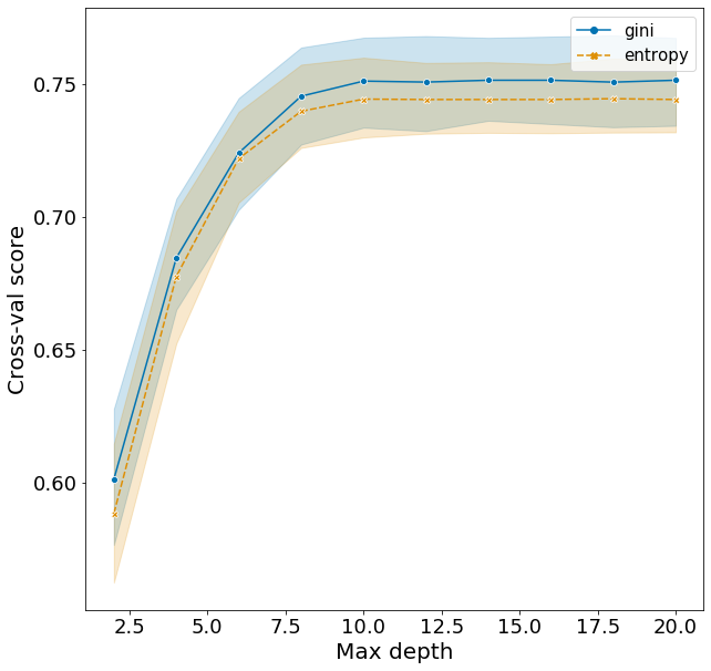
Explore hyperparameters
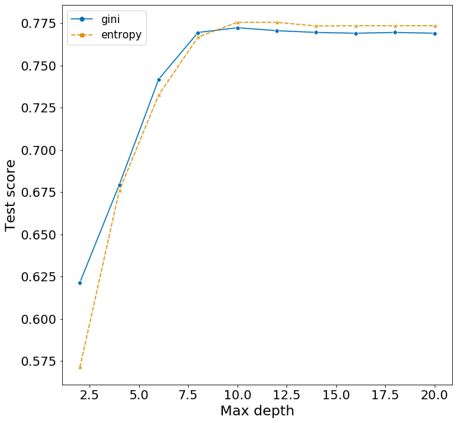
Here I explore the effects of criterion and max_depth on F1, fixing the other variables according to the best model above. The range of hyperparameters I examined are listed below, but I won’t repeat the code for obtaining the F1 scores.
# Parameters
min_samples_split, min_samples_leaf = 60, 10
list_criterion = ['gini', 'entropy']
list_max_depth = [2,4,6,8,10,12,14,16,18,20]
Plotting these scores show some interesting patterns.
- Increasing max_depth from 2 to 10 raises F1 very quickly.
- There is evidence of overfitting. The optimal model from hyperparameter tuning suggests using the criterion gini. This is observed in the cross-validation scores, however the test score is actually lower when using gini compared to entropy. This suggest that using the slightly less optimal model with the entropy criterion would avoid some of this overfitting to the training set and make better predictions for the test set.
Random forest classifier
Hyperparameter tuning
Fine-tune criterion, n_estimators, max_depth, min_samples_split, and min_samples_leaf. Utilize StratifiedKFold for cross-validation with 3 folds. Perform randomized grid search with 200 iterations which amounts to 600 fits after accounting for cross-validation. Note that the range of hyperparameter value shown here are the results of slowly narrowing the range based on several rounds of randomized search.
# Define model. cross-val, parameters
model = RandomForestClassifier()
cv = StratifiedKFold(n_splits=3)
parameters = {
    'criterion':['gini','entropy'],
    'n_estimators': [200, 300, 400, 500],
    'max_features': ['sqrt', 'log2'],
    'max_depth': [20, 30, 40, 50, 60],
    'min_samples_split': [5,10,15,20],
    'min_samples_leaf': [2,4,6,8,10]}
scoring = make_scorer(f1_score)
n_iter = 200
# Randomized search
random_search_wrapper(model, parameters, cv, scoring, n_iter=n_iter)
The best model has a training F1 of 0.809 and a test F1 of 0.817.
Best parameters:  {'n_estimators': 300, 'min_samples_split': 5, 'min_samples_leaf': 2, 'max_features': 'sqrt', 'max_depth': 40, 'criterion': 'gini'}
Best score:  0.8085174923910863
Confusion matrix:
 [[3494  206]
 [ 479 1527]]
F1: 0.8167959347419096
Accuracy: 0.8799509288468279
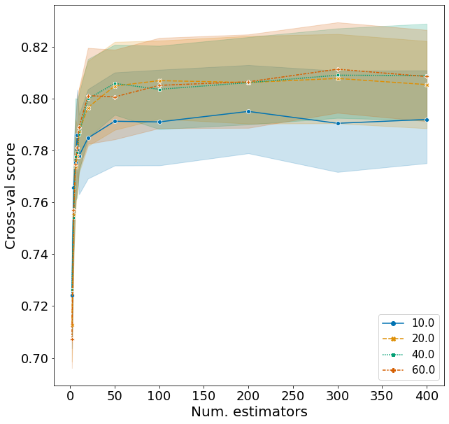
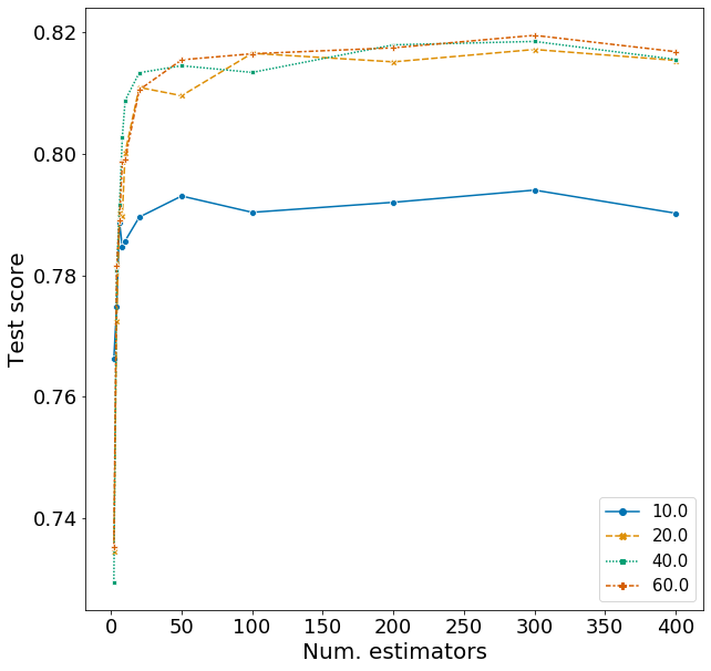
Explore hyperparameters
Here I explore the effects of n_estimators and max_depth on F1, fixing the other variables according to the best model above. The range of hyperparameters I examined are listed below, but I won’t repeat the code for obtaining the F1 scores.
# Parameters
criterion, min_samples_split, min_samples_leaf, max_features = 'entropy', 5, 2, 'sqrt'
list_n_estimators = [2,4,6,8,10,20,50,100,200,300,400]
list_max_depth = [10,20,30,40,50,60]
Plotting these scores show some interesting patterns.
- Although the optimal n_estimators is 300, we can obtain a high F1 with just around 50 trees. Running 50 rather than 300 trees can save a lot of time.
- Similarly, a high F1 score is obtained once max_depth is larger than 10. There is not much difference when setting max_depth to 20, 40, or 60.
Neural network classifier
Hyperparameter tuning
Fine-tune hidden_layer_sizes, activation, solver, alpha, and learning_rate. Utilize StratifiedKFold for cross-validation with 3 folds. Perform grid search on 288 models which amounts to 864fits after accounting for cross-validation. Note that the range of hyperparameter value shown here are the results of slowly narrowing the range based on several rounds of grid search.
I will only be testing networks with one and two hidden layers. As will be shown later, adding a second hidden layer does not improve the performance of the classifier very much.
# Define model. cross-val, parameters
model = MLPClassifier()
cv = StratifiedKFold(n_splits=3)
parameters = {
    'hidden_layer_sizes': [(5),(10),(20),(5,5),(10,10),(20,20)],
    'activation': ['identity','logistic','tanh','relu'],
    'solver': ['lbfgs,''sgd', 'adam'],
    'alpha': [0.0001, 0.001, 0.01],
    'learning_rate': ['constant','adaptive'],
    'max_iter': [1000]
}
scoring = make_scorer(f1_score)
# Grid search
grid_search_wrapper(model, parameters, cv, scoring)
The best model has a training F1 of 0.804 and a test F1 of 0.811.
Best parameters:  {'activation': 'tanh', 'alpha': 0.0001, 'hidden_layer_sizes': (20, 20), 'learning_rate': 'adaptive', 'max_iter': 1000, 'solver': 'adam'}
Best score:  0.8036652051440711
Confusion matrix:
 [[3513  187]
 [ 510 1496]]
F1: 0.8110599078341013
Accuracy: 0.8778478794251665
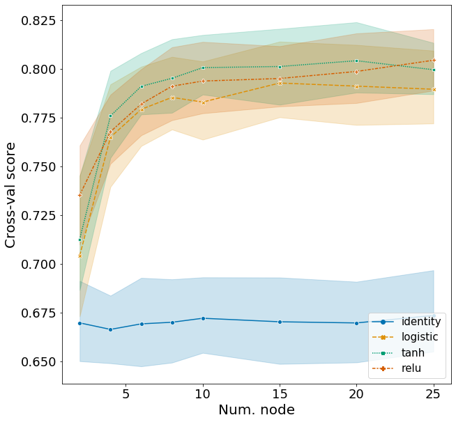
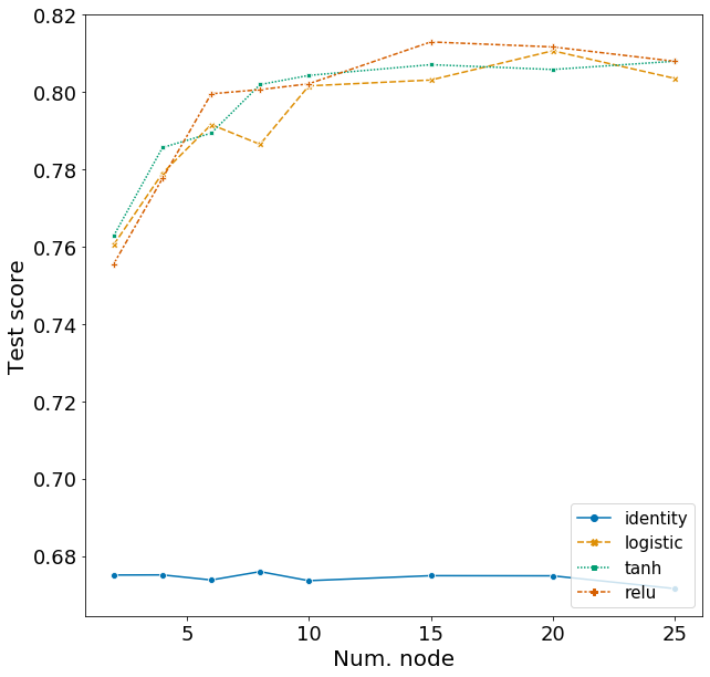
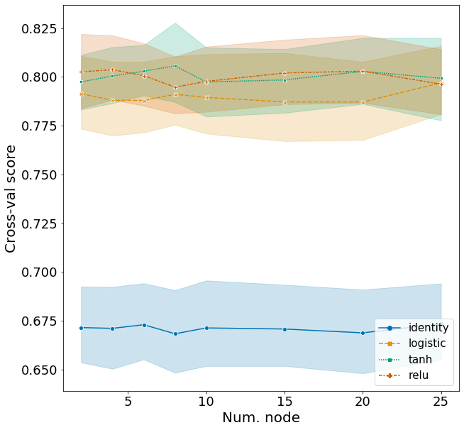
Explore hyperparameters (one hidden layers)
Here I explore the effects of activation function and the number of nodes in a network with one hidden layer. Hyperparameters for other arguments are assigned based on the best model from above. The range of hyperparameters I examined are listed below, but I won’t repeat the code for obtaining the F1 scores.
# Parameters
solver, max_iter, learning_rate, alpha = 'adam', 1000, 'adaptive', 0.0001
list_activation = ['identity','logistic','tanh','relu']
list_num_node = [2,4,6,8,10,15,20,25]

# Loop through all parameter combinations
for activation in list_activation:
    for num_node in list_num_node:
        # one hidden layer with num_node nodes
        hidden_layer_sizes = (num_node)
       '''
       Code for obtaining scores not repeated here
       '''
Plotting these scores show some interesting patterns.
- The identity activation function performs far worse then the other activation functions.
- F1 score increases sharply from 2 to 10 nodes and plateaus afterwards.
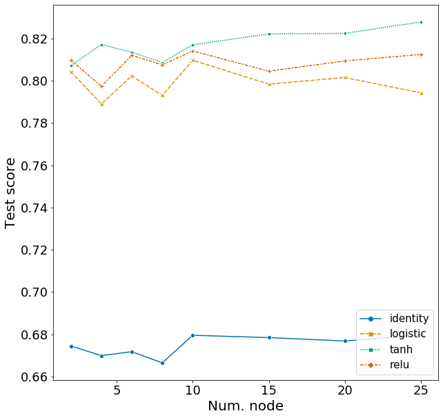
Explore hyperparameters (two hidden layers)
Here I explore the effects of activation function and the number of nodes in a network with two hidden layers. I will set the number of nodes in the first layer as 20 and vary the number of nodes in the second layer. Hyperparameters for other arguments are assigned based on the best model from above.
# Parameters
solver, max_iter, learning_rate, alpha = 'adam', 1000, 'adaptive', 0.0001
list_activation = ['identity','logistic','tanh','relu']
list_num_node = [2,4,6,8,10,15,20,25]

# Loop through all parameter combinations
for activation in list_activation:
    for num_node in list_num_node:
        # two hidden layers with num_node nodes in second layer
        hidden_layer_sizes = (20, num_node)
        '''
        Code for obtaining scores not repeated here
        '''
Plotting these scores show some interesting patterns.
- The identity activation function performs far worse then the other activation functions.
- The number of nodes in the second layer has very effect on F1, but does have a higher score than models with just one hidden layer.
- With two hidden layers, the tanh activation function is clearly the best model, followed by relu and logistic (based on test scores). This was less clear in the model with one hidden layer.
Conclusions
| Classifier | Training F1 | Test F1 | Test accuracy |
|---|---|---|---|
| Nearest neighbor | 0.736 | 0.743 | 0.843 |
| Decision tree | 0.762 | 0.772 | 0.850 |
| Random forest | 0.809 | 0.817 | 0.880 |
| Neural network | 0.804 | 0.811 | 0.878 |
It seems that the more complex random forest ensemble classifier and the neural network performed better than the nearest neighbor and decision tree classifiers. This is true when looking at both the F1 and the accuracy score.
Exploring the effects of hyperparameters on the F1 score revealed some interesting findings.
- The optimal model found by grid/randomized search may give the best score, but may do so at the cost of longer processing time. The optimal random forest model utilized 300 estimators, but 50 to 100 estimators is achieves a similar score and would save processing time (Figure 7). The optimal neural network contains two hidden layers, but one hidden layer achieves a similar score and would save processing time (Figure 8, 9).
- Hyperparameter tuning can lead to overfitting that is not obvious by just looking at the training and test score of the optimal model. The optimal decision tree utilizes the Gini impurity to measure information gain, rather than entropy. However, when we explored using the entropy criterion, we find that it has a lower score when fitted on the training set, but ultimately has a slightly higher score on the test set (Figure 6)
Throughout this analysis, I have not considered the consequences of false positive (FP) versus false negative (FN) predictions. There are many studies that aim to minimize FN more than FP or vice versa. For example, in disease prediction, a FN may be more consequential than a FP because a FN would mean a disease becomes untreated, while a FP may just warrant further testing. For our analysis, I would aim to reduce FP more than FN because accepting a hadronic event as a gamma ray event can be very misleading. To account for these considerations, I will continue exploring this dataset using AUC-ROC curves in Part 2 of this analysis
Image credits: Unsplash, https://www.isdc.unige.ch/cta/outreach