I concluded in Part 1 of this analysis with four types of classifiers, each optimized by fine-tuning hyperparameters. From these results, it is clear that the random forest and neural network classifier are preferable to nearest neighbor and decision tree.
| Classifier | Training F1 | Test F1 | Test accuracy |
|---|---|---|---|
| Nearest neighbor | 0.736 | 0.743 | 0.843 |
| Decision tree | 0.762 | 0.772 | 0.850 |
| Random forest | 0.809 | 0.817 | 0.880 |
| Neural network | 0.804 | 0.811 | 0.878 |
The Decision Threshold
Tuning the input is essential for building a good classifier, but it is equally important to study and tune the output. The output of a classifier is typically the probability assessment of a class. This probability is then used to bin the data point into a class based on a decision threshold. In most classifiers the default decision threshold is set at t = 0.5, such that the data point is classified as ‘0’ if its class probability is below 0.5 and classified as ‘1’ otherwise.
It should be obvious now that the value of t can have large consequences on the predicted class, especially when class probabilities are noisy and hover around 0.5. This would impact whether the prediction is a false positive (FP), false negative (FN), true positive (TP), or true negative (TN). The count of these prediction types can be displayed on a confusion matrix.
| Predict positive | Predict negative | |
|---|---|---|
| Actual positive | TP | FN |
| Actual negative | FP | TN |
Example
Below is an example of how t may or may not affect predictions. The Probability and Actual columns represent the class probability output by the classifier and the actual class of the data point, respectively. The Prediction-0.5 and Result-0.5 columns represent the prediction and result when setting the decision threshold at t = 0.5 (analogous for Prediction-0.6 and Result-0.6). In the first four rows, adjusting t has no effect because the class probabilities are either below 0.5 or above 0.6. In the fifth row, adjusting t to 0.6 changes the result from being a FP to a TN. In the sixth row, adjusting t to 0.6 changes the result from a TP to a FN.
| Probability | Actual | Prediction-0.5 | Prediction-0.6 | Result-0.5 | Result -0.6 |
|---|---|---|---|---|---|
| 0.82 | 1 | 1 | 1 | TP | TP |
| 0.07 | 0 | 0 | 0 | TN | TN |
| 0.68 | 0 | 1 | 1 | FP | FP |
| 0.22 | 1 | 0 | 0 | FN | FN |
| 0.58 | 0 | 1 | 0 | FP | TN |
| 0.55 | 1 | 1 | 0 | TP | FN |
FPR and TPR
Rather than counting each type of prediction in the confusion matrix, it is typical to calculate the false positive rate (FPR) and true positive rate (TPR). The FPR represents the proportion of actual negative events that were correctly predicted as negative events: FPR = FP /(FP+TN). The TPR represents the proportion of actual positive events that were correctly predicted as positive events: TPR = TP / (FN+TP).
Depending on the needs of your project, you can tune the decision threshold, t, and optimize for the FPR and/or TPR. For example, in disease detection, you may want to maximize the TPR (i.e. reduce the FNR = 1 - TPR) because missing a positive detection can be much more consequential then falsely detecting disease presence (which would just warrant a second test to check).
Below, I will examine the effects of adjust t on each of our four classifiers. In an actual study on gamma ray detection, one may prefer to optimize for low FPR at the cost of reduced TPR because there are typically many more hadronic events than gamma ray events in real data. Imagine that there are 10,000 hadronic events and only 100 gamma events. If an adjustment in t causes a reduction in FPR and TPR by 1%, this would reduce 100 false positives at the cost of 1 true positive.
Python packages and functions
import numpy as np
import pandas as pd
import seaborn as sns
import matplotlib.pyplot as plt
from sklearn.model_selection import train_test_split, cross_val_score,  StratifiedKFold

from sklearn.neighbors import KNeighborsClassifier
from sklearn.tree import DecisionTreeClassifier
from sklearn.ensemble import RandomForestClassifier
from sklearn.neural_network import MLPClassifier
from sklearn.metrics import confusion_matrix, plot_roc_curve, roc_auc_score, roc_curve
def adjPred(Y_proba, t):
    """
    Adjusts class predictions based on the decision threshold (t)
    """
    return [1 if y >= t else 0 for y in Y_proba[:,1]]

def calcFprTpr(Y_test, Y_proba, t):
    '''
    Get FPR and TPR given decision threshold
    '''
    Y_pred = adjPred(Y_proba, t) #get adjusted predictions
    tn, fp, fn, tp = confusion_matrix(Y_test, Y_pred).ravel() #get confusion matrix metrics
    fpr, tpr = fp/(fp+tn), tp/(tp+fn)
    return [tn, fp, fn, tp, fpr, tpr]

def tableFprTpr(Y_test, Y_proba, listT):
    '''
    Generate table of FPR, TPR with user-defined sequence of thresholds
    '''
    dfRates = pd.DataFrame(columns=['Threshold','TN','FP','FN','TP','FPR','TPR'])
    for t in listT:
        tn, fp, fn, tp, fpr, tpr = calcFprTpr(Y_test, Y_proba, t)
        dfRates.loc[len(dfRates)] = [t, tn, fp, fn, tp, fpr, tpr]
    return dfRates

def thresholdGivenFpr(Y_test, Y_proba, maxFPR):
    '''
    Find the largest decision threshold (t) that returns FPR <= maxFPR
    '''
    for t in list(np.linspace(0,1,1001)):
        tn, fp, fn, tp, fpr, tpr = calcFprTpr(Y_test, Y_proba, t)
        if fpr <= maxFPR:
            return [tn, fp, fn, tp, fpr, tpr, t]
Define classifiers
Read the csv data file
Telescope = pd.read_csv('telescope.csv')
Encode class identifier (Y), split the data into training and test set, and standardize features (X).
# Define X as features and Y as labels
X = Telescope.drop('class', axis=1)
Y = Telescope['class']
# Encode Y
le = LabelEncoder()
Y_encode = le.fit_transform(Y)
# split to training and testing set, stratify by Y
X_train, X_test, Y_train, Y_test = train_test_split(X, Y_encode, test_size=0.30, stratify=Y)
# Standardize X_train, then fit to X_test
scaler = StandardScaler()
scaler.fit(X_train)
X_train = scaler.transform(X_train)
X_test = scaler.transform(X_test)
Define the four classifiers based on the fine-tuned hyperparameters from Part 1. Fit each classifier with training data. Obtain predictions using the default decision threshold (t = 0.5). Obtain the class probabilities for each data point using predict_proba. These class probabilities will be used to make predictions when we alter the decision threshold, t.
#####-----nearest neighbors
NN = KNeighborsClassifier(p=1, weights='distance', n_neighbors=5)
NN.fit(X_train, Y_train)
NN_Y_pred = NN.predict(X_test)
NN_Y_proba = NN.predict_proba(X_test)

#####-----decision tree
DT = DecisionTreeClassifier(criterion='gini', max_depth=10, min_samples_split=60, min_samples_leaf=10)
DT.fit(X_train, Y_train)
DT_Y_pred = DT.predict(X_test)
DT_Y_proba = DT.predict_proba(X_test)

#####-----random forest
RF = RandomForestClassifier(criterion='gini', max_features='sqrt', max_depth=40, n_estimators=300,min_samples_split=5, min_samples_leaf=2)
RF.fit(X_train, Y_train)
RF_Y_pred = RF.predict(X_test)
RF_Y_proba = RF.predict_proba(X_test)

#####-----neural network
MLP = MLPClassifier(activation='tanh', solver='adam', hidden_layer_sizes=(20,20), max_iter=1000, learning_rate='adaptive', alpha=0.0001)
MLP.fit(X_train, Y_train)
MLP_Y_pred = MLP.predict(X_test)
MLP_Y_proba = MLP.predict_proba(X_test)
Examining class probabilities
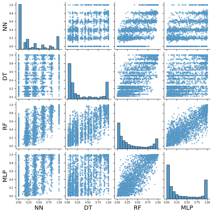
Before even considering the decision threshold, lets take a look at the class probabilities assigned by each classifier.
As expected, class probabilities range from 0 to 1. However, we observe that the neural network and decision tree classifiers assigns probability of 1 much more often than the random forest and neural network classifiers.
dfProb = pd.DataFrame({'NN':NN_Y_proba[:,1],'DT':DT_Y_proba[:,1],'RF':RF_Y_proba[:,1],'MLP':MLP_Y_proba[:,1]})
print(dfProb.describe().loc[['count','mean','std','min','50%','max']])
                NN           DT           RF          MLP
count  5706.000000  5706.000000  5706.000000  5706.000000
mean      0.296769     0.349363     0.348438     0.359866
std       0.363212     0.372850     0.347748     0.385066
min       0.000000     0.016760     0.000000     0.000058
50%       0.179352     0.138983     0.195281     0.158873
max       1.000000     1.000000     1.000000     0.999994
print(sum(temp0.NN==1),sum(temp0.DT==1),sum(temp0.RF==1),sum(temp0.MLP==1))
758 667 39 0
We also observe that the correlation in class probabilities are lower when considering the nearest neighbor classifier, and highest between random forest and neural network classifiers.
dfCorrProb = dfProb.corr()
           NN        DT        RF       MLP
NN   1.000000  0.823648  0.897634  0.855501
DT   0.823648  1.000000  0.918581  0.862727
RF   0.897634  0.918581  1.000000  0.944070
MLP  0.855501  0.862727  0.944070  1.000000
Histogram of class probabilities show bimodal distributions with peaks at 0 and near 1. However the large number of points with intermediate probabilities suggests that adjusting the threshold value will have significant effects on class assignments.
sns.set_context("paper", rc={"axes.labelsize":20})
sns.pairplot(dfProb, height = 2.5, plot_kws={'alpha':0.5})
Varying the decision threshold
Before we attempt to optimize the classifiers, lets examine the effects of altering the decision threshold, t, on the false positive rate (FPR) and true positive rates (TPR). Although this data is usually represented in a ROC-curve (below), plotting FPR and TPR against values of t helped me understand this process a bit more easily.
To classify data points in the test set using a custom decision threshold, I utilize adjPred (defined above), which categorized the data point as ‘0’ if the class probability is below t, and as ‘1’ otherwise.
listI, listJ, listTitle =[0,0,1,1], [0,1,0,1], ['Nearest neighbor','Decision tree','Random forest','Neural network']
listT, listProba = list(np.linspace(0,1,501)), [NN_Y_proba, DT_Y_proba, RF_Y_proba, MLP_Y_proba]

# loop to produce subplots
fig, ax =plt.subplots(2, 2, figsize=(26,20))
fig.subplots_adjust(hspace=0.2, wspace=0.1)
for k in range(4):
    # table of FPR, TPR for range of decision thresholds
    model_rates = tableFprTpr(Y_test, listProba[k], listT)
    model_rates_melt = pd.melt(model_rates, id_vars=['Threshold'], value_vars=['FPR', 'TPR'], var_name='Type', value_name='Rate')
    sns.lineplot(
        data=model_rates_melt, x='Threshold', y='Rate', hue='Type', style='Type',
        palette="colorblind", markers=True, ax=ax[listI[k],listJ[k]])
    ax[listI[k],listJ[k]].vlines(x=0.5, ymin=0, ymax=1, color='black', linestyle='--', alpha=0.8)
    ax[listI[k],listJ[k]].set_title(listTitle[k], fontsize=20, loc='left')
    ax[listI[k],listJ[k]].set_xlabel(xlabel='Threshold',fontsize=20)
    ax[listI[k],listJ[k]].set_ylabel(ylabel='Rate', fontsize=20)
    ax[listI[k],listJ[k]].tick_params(axis='both', which='major', labelsize=18)
    ax[listI[k],listJ[k]].legend(loc='upper right', prop={'size': 30})
plt.show()
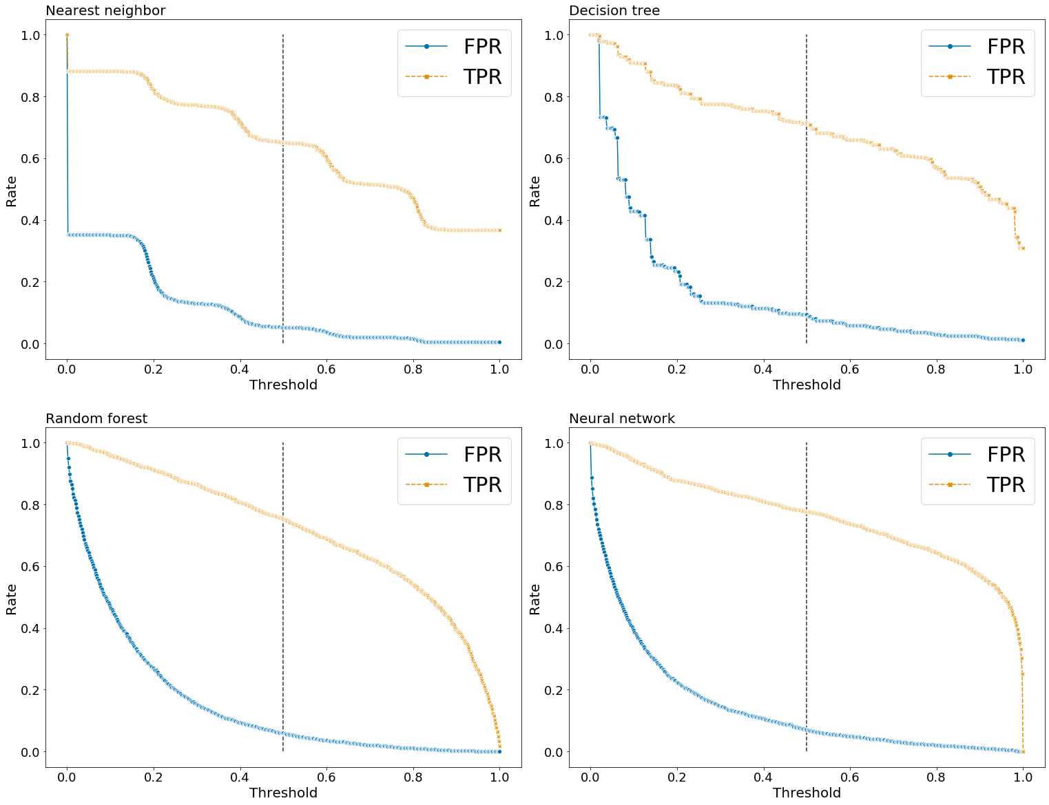
Here is what I learned from examining these plots. Recall the FPR = FP/(FP+TN) and TPR = TP/(FN+TP).
- FPR = 1 and TPR = 1 when t = 0, since TN = 0 and FN = 0.
- When t = 1, the TPR for nearest neighbor and decision tree classifiers are well above 0, while the TPR for the random forest and neural network classifiers are at or near 0. This is expected given that the former two classifiers assigned many more data points a class probability equal to 1. However, exactly why this is the case is not clear to me.
- As expected, FPR and TPR decreases as t increases, but the shape of the curve differs across classifiers. For the nearest neighbor classifier, there is a step-like curve suggesting that the class probabilities cluster around a few values (which is actually observed in the histogram above). The decision tree classifier show a similar but less pronounced step-like curve. The random forest and neural network classifier shows a smoother curve.
- Interestingly, for the random forest and neural network classifier, the FPR show a negative curvature, while the TPR show a positive curvature. This means that for small values of t, as t increase, the FPR decreases at a faster rate than the TPR. While for larger value of t, as t increases the TPR rate decreases faster than the FPR.
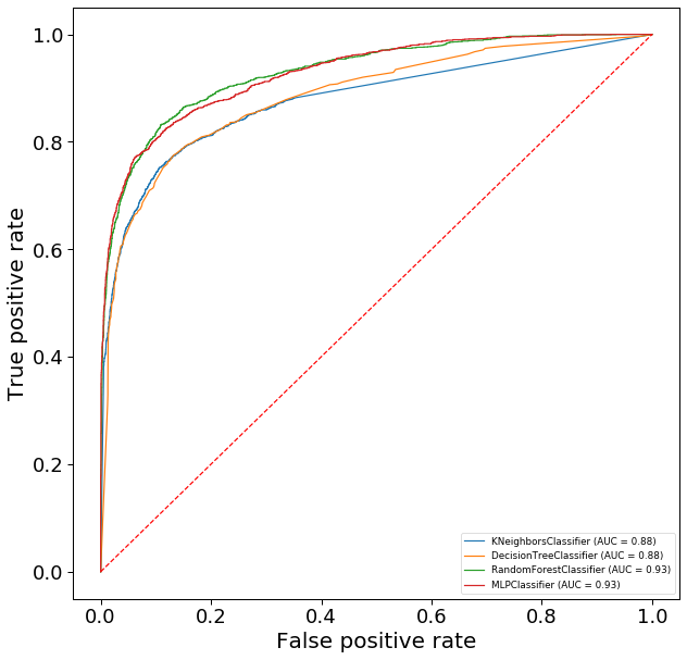
ROC curves
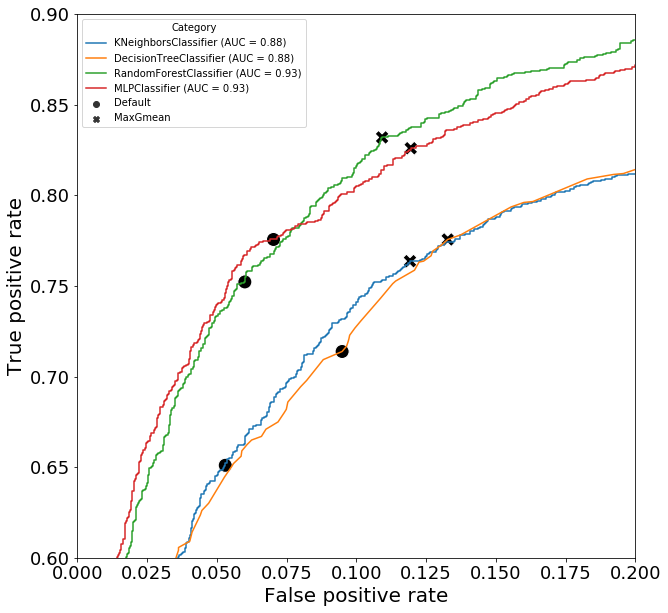
Here, we will plot the receiver operating characteristic (ROC) curve, which is simply a plot of FPR against TPR for a range of decision thresholds. This curve typically exhibits a positive curvature, showing that TPR is larger than FPR. Importantly, the area under the curve (AUC) can be used to score a classifier model. A larger AUC-ROC score suggests a model with a better fit to the data.
The plot below shows the ROC-curve and the AUC-ROC score for all four classifiers. We observe the classical positive curvature for all four classifiers, but also that the AUC is larger for the random forest and neural network classifiers (0.93) compare to the nearest neighbor and decision tree classifiers (0.88). In other words, similar to the accuracy and F1 score, the AUC-ROC score would rank the random forest and neural network classifiers as a better model for the data.
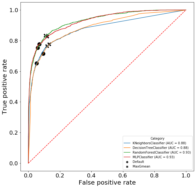
Geometric mean optimization of t
So far, we have just examined various properties of the class probabilities and decision thresholds. Here, we will attempt to find the optimal decision threshold, t, for each model using the geometric mean method. This method simply aims to finds the value of t that maximizes the geometric mean of sensitivity (TPR) and specificity (1 - FPR), which turns out to equal sqrt(TPR * (1-FPR)).
# Find value of t that maximized geometric mean
listProba = [NN_Y_proba, DT_Y_proba, RF_Y_proba, MLP_Y_proba]
listName = ['Nearest neighbor','Decision tree','Random forest','Neural network']

dfGmean = pd.DataFrame(columns=['Model','Category','Threshold','FPR','TPR'])
for i in range(4):
    # -get point for threshold=0.5
    tn, fp, fn, tp, fpr, tpr = calcFprTpr(Y_test, listProba[i], 0.5)
    dfGmean.loc[len(dfGmean)] = [listName[i], 'Default', 0.5, fpr, tpr]
    # get point for maximum gmean
    fpr, tpr, thresholds = roc_curve(Y_test, listProba[i][:,1])
    gmeans = np.sqrt(tpr * (1-fpr))
    ix = np.argmax(gmeans)
    dfGmean.loc[len(dfGmean)] = [listName[i], 'MaxGmean', thresholds[ix], fpr[ix], tpr[ix]]
We observe that the optimized value of t has a lower value that the default across all four classifiers. Although lowering the threshold increases TPR, it also increases the FPR. Looking at the results for the random forest classifier, reducing t from 0.5 to 0.36 causes a 0.08 increase in TPR and a 0.049 increase in FPR. However this is actually an increase of 11% for the TPR and an increase of 82% for the FPR.
This is not always ideal, especially with unbalanced datasets containing many more negative events than positive events, which is almost always the case when detecting gamma ray events (most event will be the ‘negative’ hadronic events).
             Model  Category  Threshold       FPR       TPR
0  Nearest neighbor   Default   0.500000  0.052973  0.651047
1  Nearest neighbor  MaxGmean   0.357613  0.119189  0.763709
2     Decision tree   Default   0.500000  0.094865  0.713858
3     Decision tree  MaxGmean   0.310345  0.132703  0.775673
4     Random forest   Default   0.500000  0.060000  0.752243
5     Random forest  MaxGmean   0.363560  0.109189  0.832004
6    Neural network   Default   0.500000  0.070270  0.775673
7    Neural network  MaxGmean   0.362441  0.119459  0.826022
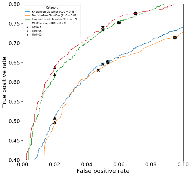
Manual optimization of t
Rather than relying on a generic method of optimization, like the geometric means method, it is typical to adjust t until an acceptable level of FPR and/or TPR is achieved. For this project, I am aiming to reduce FPR to low levels since hadronic events are typically much more abundant than gamma ray events. It would be ideal to maximally reduce false positives, while still achieve significant true positive rates.
Here I will find the value of t that would achieve a FPR of 5% or 2% and examine how this affects the TPR. I have defined a simple function thresholdGivenFpr to do this.
listProba = [NN_Y_proba, DT_Y_proba, RF_Y_proba, MLP_Y_proba]
listName = ['Nearest neighbor','Decision tree','Random forest','Neural network']

dfManual = pd.DataFrame(columns=['Model','Category','Threshold','FPR','TPR'])
for i in range(4):
    #####-----get point for threshold=0.5
    tn, fp, fn, tp, fpr, tpr = calcFprTpr(Y_test, listProba[i], 0.5)
    dfManual.loc[len(dfManual)] = [listName[i], 'Default', 0.5, fpr, tpr]
    #####-----get point for FPR=0.05
    tn, fp, fn, tp, fpr, tpr, t = thresholdGivenFpr(Y_test, listProba[i], 0.05)
    dfManual.loc[len(dfManual)] = [listName[i], 'Fpr0.05', t, fpr, tpr]
    #####-----get point for FPR=0.01
    tn, fp, fn, tp, fpr, tpr, t = thresholdGivenFpr(Y_test, listProba[i], 0.02)
    dfManual.loc[len(dfManual)] = [listName[i], 'Fpr0.01', t, fpr, tpr]
We observe that when optimizing for low FPR, the decision threshold t increases relative to the default value, which is opposite to what happened when optimization using the geometric mean. Of course, lowering the FPR comes at the cost of a lower TPR and it is up to the analyst to decide how much of the TPR they are willing to sacrifice. Looking at the results of the random forest classifier, reducing FPR to 0.05 reduced FPR by 17% and TPR by just 3%, while reducing FPR to 0.02 reduced FPR by 67% and TPR by 18%.
               Model Category  Threshold       FPR       TPR
0   Nearest neighbor  Default      0.500  0.052973  0.651047
1   Nearest neighbor  Fpr0.05      0.548  0.050000  0.645563
2   Nearest neighbor  Fpr0.02      0.758  0.020000  0.507976
3      Decision tree  Default      0.500  0.094865  0.713858
4      Decision tree  Fpr0.05      0.667  0.047027  0.630110
5      Decision tree  Fpr0.02      0.901  0.020000  0.497009
6      Random forest  Default      0.500  0.060000  0.752243
7      Random forest  Fpr0.05      0.530  0.050000  0.733300
8      Random forest  Fpr0.02      0.711  0.020000  0.619143
9     Neural network  Default      0.500  0.070270  0.775673
10    Neural network  Fpr0.05      0.595  0.050000  0.740279
11    Neural network  Fpr0.02      0.810  0.020000  0.637089
Conclusions
Optimizing the decision threshold for a classifier model can be a very important step to alter the FPR/TPR to levels that are acceptable for the project, especially for unbalanced datasets. As shown above, blindly using a standard approach, such as optimizing by geometric mean, can be detrimental to your project specifications.
It is also important to understand that optimizing for the decision threshold would change all the other scores, since they are based on the metrics on the confusion table. The table below shows how optimizing t affects the accuracy and F1 score in our random forest model.
| Optimization | t | FPR | TPR | Test accuracy | Test F1 |
|---|---|---|---|---|---|
| Default | 0.50 | 0.056 | 0.761 | 0.880 | 0.817 |
| Geometric mean | 0.340 | 0.129 | 0.863 | 0.868 | 0.821 |
| FPR=0.05 | 0.509 | 0.05 | 0.757 | 0.882 | 0.819 |
| FPR=0.02 | 0.685 | 0.02 | 0.637 | 0.859 | 0.761 |