This post contains my notes on decision tree classifiers and regressors. I have split my notes into two parts. The first part will describe the methodology constructing decision trees along with some of the mathematics involved. The second part will be more code heavy and involve step-by-step construction of a decision tree using the algorithm described by scikit-learn.
Decision tree
Decision trees are a non-parametric supervised learning method for classification and regression. The goal is to create a model that learns a hierarchy of if/else questions, using the data features to predict the value of the target variable. Decision trees can be used for categorical and continuous target variables. They are relatively simple to understand and can be easily visualized using a decision tree.
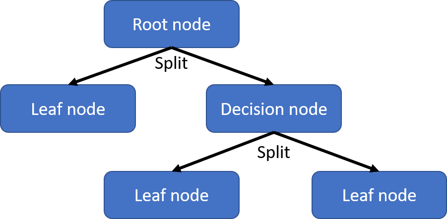
It is useful to first learn about the different parts of a decision tree. At the top is the root node, which is the starting point and represents the entire dataset. At each step, the dataset is split into two (or more) sub-nodes based on the particular value of one of its features. Which features to utilize and what values to split the data points on is the main challenge on constructing the model. There are numerous algorithms that can be used and one of the most popular is the classification and regression tree (CART) algorithm, which will be discussed in detail in the rest of these notes. After a split, the resulting sub-nodes can either be a leaf (terminal) node or a decision node. The leaf node represents an end to a tree and will not be subject to further splitting. Decision nodes represents one where further splitting will occur. You can actually think of the root node as just the first decision node of the tree.
Building a decision tree
- Begin with the entire dataset at the root node.
- Search over all possible splits and find the one that is most informative about the target; each split only concerns one feature. A split typically involves splitting the data base on whether its feature value is <= or > than a threshold value. The aim is to find the split that minimized the impurity of the sub-nodes. Thus, most decision tree algorithms are greedy algorithm that find the local optimum solution at each node, but this does not necessarily lead to a globally optimal decision tree.
- Use the most informative split (minimum impurity) to divide the dataset into “left” and “right” sub-nodes.
- Repeat steps 2 and 3 to recursively partition the dataset until each leaf only contains a single target class / regression value. A leaf node containing only data points with the same target value is a called pure. However, a leaf node can be impure for at least two reasons. Firstly, there may simply not be enough information in the features to separate data points with different target values. Secondly, construction of the tree may be halted if some restriction is met to reduce overfitting (e.g. maximum depth was reached).
Prediction
Once a decision tree is learned from training on the data, a prediction is made for new data points by looking at which leaf node they fall on based on their feature values. The prediction for the leaf node is simply the majority target for decision tree classifiers or the mean value of targets for decision tree regressors. Note that for decision tree regressors, the predicted value will never be outside of the values in the training dataset (i.e. it does not extrapolate).
An addition note for scikit-learn users using DecisionTreeClassifier. After a model is trained, the predict method is giving the majority target at the leaf node. The predict_proba method will output the proportion of each target class in the leaf node.
Measures of impurity
Evaluating the impurity of nodes is essential for building a decision tree. After all, the goal is to find the combination in feature space that would accurately predict the target value (minimize impurity). If the leaf node is highly impure, then the decision path that led to it would not give accurate predictions. It is important to separate the impurity of a node from the quality of the split. The former is calculated based on the target variables in a single node, while the latter is calculated using the impurity of sub-nodes (and sometimes the parent node) of a split. I will discuss how impurity is calculated here and the quality of the split in a later section.
Here I will define the impurity function as \(H(S_{m})\), where \(S_{m}\) represents the set of data points at node \(m\). Impurity will obviously be calculated different for categorical vs continuous target variables. I will only present a few common measures here.
Classification measures of impurity
Given a categorical target variable with (k\) classes (0, 1, …, k-1, k). Let the proportion of each class at leaf node \(m\) be \(p_{m, k}\).
Gini index
The Gini index is used by the CART algorithm. It measures how often a randomly chosen data point in the node would be incorrectly labeled. A pure and a maximumally impure node will have Gini index values of 0 and 0.5, respectively.
\[\begin{aligned} H(S_{m}) &=\sum_{k} p_{m,k}(1-p_{m,k}) \\ &=\sum_{k} p_{m,k}-\sum_{k} p_{m,k}^{2} \\ &=1-\sum_{k} p_{m,k}^{2} \end{aligned}\]Entropy
Entropy is a measure of disorder, which increases with increasing abundances of data points with different target values. A pure and a maximallay impure node will have entropy values of 0 and 0.5, respectively.
\[H(S_{m}) =-\sum_{k} p_{m,k}\log_{2}p_{m,k}\]Example
If we assume that the dataset only has two classes (0 and 1). At node \(m\) the proportion of data of class 0 and class 1 will be \(p_{0}\) and \(p_{1}=1-p_{0}\), respectively. For this type of data, we can examine the Gini and entropy curve for all values of \(p_{0}\) from 0 to 1.
from math import log
import numpy as np
import pandas as pd
import seaborn as sns

def gini_index(p0):
    '''
    Calculate gini index for binary target variable
    '''
    p1 = 1-p0
    return 1 - (p0**2 + p1**2)

def entropy(p0):
    '''
    Calculate entropy for binary target variable
    '''
    p1 = 1-p0
    try:
        return (-1 * (p0 * log(p0, 2) + p1 * log(p1, 2)))
    except ValueError:
        return 0

# create lists of p0, Gini and Entropy
listP0 = list(np.arange(0,1+0.01,0.01))
listGini = [gini_index(p0) for p0 in listP0]
listEntropy = [entropy(p0) for p0 in listP0]
# create dataframe
dfImpurity = pd.DataFrame({
    'p0':listP0+listP0+listP0,
    'measure':['p0']*len(listP0)+['Gini']*len(listGini)+['Entropy']*len(listEntropy),
    'impurity':listP0+listGini+listEntropy
})
# plot using seaborn
fig, ax = plt.subplots(figsize=(8, 8))
sns.lineplot(
    data=dfImpurity, x='p0', y='impurity',
    hue='measure', palette="colorblind", markers=True)
ax.set_xlabel(xlabel='Proportion of class 0',fontsize=20)
ax.set_ylabel(ylabel='Impurity', fontsize=20)
ax.tick_params(axis='both', which='major', labelsize=18)
ax.legend(prop={'size': 15})
plt.show()
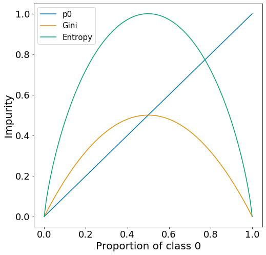
For both measures of impurity, there is a peak at \(p_{0} = 0.5\), which represents a node with maximal impurity. Impurity then approaches 0 as \(p_{0}\) approaches 0 and 1, which represents nodes with only class 0 or only class 1 target variables.
Regression measures of impurity
Given a continuous target variable at node \(m\) with \(N_{m}\)values represented by vector \(y\), let \(\bar{y}\) be the mean and \(\tilde{y}\) be the median of vector y.
Mean squared error (MSE)
Measure squared error has many applications, especially in statistical regressions. It is a useful statistic to measure the variation of a random variable around a mean. The minimum value of the MSE is 0, but there is no upper limit (unlike Gini and Entropy).
\[H(S_{m}) = \frac{1}{N_{m}} \sum_{y} (y-\bar{y})^{2}\]Mean absolute error (MAE)
The mean absolute error is less commonly used. However it is less sensitive to outlier data points compared to the mean squared error. The one drawback is that determining the median of a vector is more computationally intensive than calculating the mean, especially when the data set is very large. The minimum value of the MAE is 0, but there is no upper limit (unlike Gini and Entropy).
\[H(S_{m}) = \frac{1}{N_{m}} \sum_{y} |y-\tilde{y}|\]Example
The example shown here is mostly meaningless. It is here just to show that you can apply the concepts of MSE and MAE to categorical target variables and to show how the plots of MSE and MAE differ from Gini and Entropy. There really is not a generalized way of showing what MSE and MAE curves may look like because it depends entirely on the values of the dataset.
Let’s assume that the dataset only has two classes (0 and 1) and there are 100 data points at node \(m\). Let proportion of data of class 0 and class 1 will be \(p_{0}\) and \(p_{1}=1-p_{0}\), respectively. Below is the MSE and MAE curve for this particular type of data across all values of \(p_{0}\) from 0 to 1.
def mean_square_error(n, n0):
    '''
    Calculate mean square error for binary continuous variable
    '''
    n1 = n-n0
    y_list = [0]*n0 + [1]*n1
    y_mean = np.mean(y_list)
    mse = sum([(y-y_mean)**2 for y in y_list]) / n
    return mse

def mean_absolute_error(n, n0):
    '''
    Calculate mean absolute error for binary continuous variable
    '''
    n1 = n-n0
    y_list = [0]*n0 + [1]*n1
    y_median = np.median(y_list)
    mae = sum([abs(y-y_median) for y in y_list]) / n
    return mae

# create data and dataframe for MSE and MAE
listP0 = list(np.arange(0,1+0.01,0.01))
listMSE = [mean_square_error(100, int(100*p0)) for p0 in listP0]
listMAE = [mean_absolute_error(100,int(100*p0)) for p0 in listP0]
dfImpurity = pd.DataFrame({
    'p0':listP0+listP0+listP0,
    'measure':['p0']*len(listP0)+['MSE']*len(listMSE)+['MAE']*len(listMAE),
    'impurity':listP0+listMSE+listMAE
})
# plot using seaborn
fig, ax = plt.subplots(figsize=(8, 8))
sns.lineplot(
    data=dfImpurity, x='p0', y='impurity',
    hue='measure', palette="colorblind", markers=True)
ax.set_xlabel(xlabel='Proportion of class 0',fontsize=20)
ax.set_ylabel(ylabel='Impurity', fontsize=20)
ax.tick_params(axis='both', which='major', labelsize=18)
ax.legend(prop={'size': 15})
plt.savefig('images/impurity.mse.mae.png', bbox_inches='tight')
plt.show()
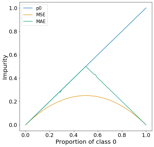
Just to repeat, this is not what a typically MSE or MAE curve would look like, this is completely specific to this type of data. MSE can be larger or smaller than MAE depending on the dataset.
Quality of the split
To evaluate the quality of a split, you would need to consider not just the impurity of a single sub-node, but the impurity at all sub-nodes created by the split and possible even the parent node. The CART algorithm considers all possible splits and keeps the split with the high quality. Similar to the impurity measures, there are various measures for the quality of the split and I will only present two of them.
Lets assume that the parent node \(m\) containing dataset \(S_{m}\) with \(N_{m}\) data points. This parent node is split into two child nodes using feature \(f\) and threshold value \(t\). The “left” child node represents the set \(S_{m}^{left}\) of \(N_{m}^{left}\) data points where \(f\) has a value <= \(t\). The “right” child node represents the set \(S_{m}^{right}\) of \(N_{m}^{right}\) data points where \(f\) has a value > \(t\).
Weighted sum of impurities
This seems to be the measure of split quality implemented by scikit-learn according to their documentation of decision trees. The quality of split at parent node \(m\) given feature \(f\) and threshold \(t\), \(G(S_{m}, f, t)\) is simply the sum of the impurities of its child nodes weighted by the proportion of data points in each child node. As far as I can tell, you can utilize \(G(S_{m}, f, t)\) to evaluate the quality of the split for categorical and continuous measures of impurities. However, I most often see this associated with the calculation of Gini impurities.
Information gain (IG)
IG is used for categorical target variables (decision tree classifiers). I mostly see it used in conjunction with Entropy but have seen a few examples of its used with Gini. IG is a measure of the difference in impurity between the parent and the child nodes after a split. Let \(E(S)\) represent the entropy of dataset \(S\) and let \(IG(S_{m}, f, t)\) be the information gain given the parent node is split by feature \(f\) using threshold \(t\).
\[IG(S_{m}, f, t) = E(S_{m}) - ( \frac{S_{m}^{left}}{S_{m}}E(S_{m}^{left})+\frac{S_{m}^{right}}{S_{m}}E(S_{m}^{right}) )\]The first term in the equation is simply the entropy of the parent node. The second term is the weighted sum of entropies in the child nodes.
Overfitting
Building a tree until all leaves are pure usually causes the model to overfit onto the training dataset. To prevent overfitting, one can perform pre-pruning to stop building the tree early on or post-pruning to remove or collapse nodes with little information. Some examples of pre-pruning include limiting the max depth of the three, limiting the maximum number of leaves, and requiring a minimum number of data point to continue splitting a node.
A related method to prevent overfitting is to utilize ensemble models of decision trees. One of the most simple and popular method is to construct random forest models. However, I will not elaborate on this in this post.