This post contains the second part of my notes on decision tree classifiers and regressors. The goal in this post is to used what I learned in Part 1 and construct a decision tree step-by-step. I will utilize the algorithm laid out by the scikit-learn documentation and check that my tree matches the tree constructed using scikit-learn.
Packages
import numpy as np
import pandas as pd
import seaborn as sns
import matplotlib.pyplot as plt
from sklearn.tree import DecisionTreeClassifier, DecisionTreeRegressor, plot_tree
from sklearn.datasets import load_iris
Simplified decision tree of Iris dataset
Here I will construct a decision tree classifier using the iris dataset. To simplify the tree, I will convert the target variable from having three classes {0: setosa, 1: versicolor, 2: virginica} to just two classes {0: not versicolor, 1: is versicolor) and limit the depth of the tree to three levels.
# load iris dataset
iris = load_iris(as_frame=True)
dfIris = iris.data
# add a new target column called 'versicolor' to indicate if sample is 'versicolor' or not
versicolor = [0 if x==1 else 1 for x in iris.target]
dfIris['versicolor'] = versicolor
We can now construct the decision tree classifier with maximum depth of three and plot the tree using the plot_tree method.
# define features and targets
features = iris.feature_names
target = 'versicolor'
# define parameters for tree
random_state = 111
max_depth = 3
# fit decision tree classifier
X, Y = dfIris[features], dfIris[target]
clf1 = DecisionTreeClassifier(random_state=111, max_depth=max_depth)
clf1 = clf1.fit(X, Y)
# plot tree
plot_tree(clf1, feature_names=features, filled=True)
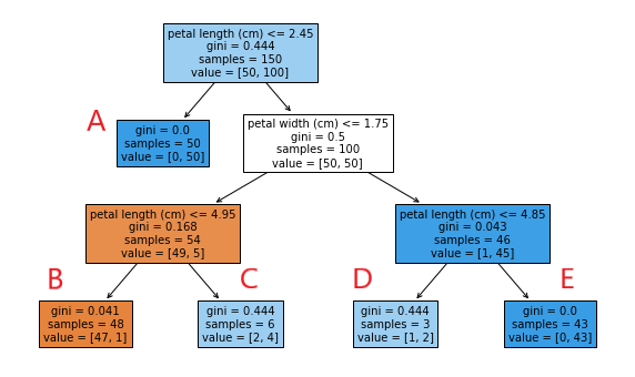
This decision tree gives you all the information you need to understand how the classifier works. For root and decision nodes, the first line indicates the feature and threshold value use to perform the split, the second gives the impurity (Gini index) of the node, the third line gives the number of samples, and the last lists the number of samples in class 0 (not versicolor) and class 1 (is versicolor). Leaf nodes are basically the same, except it does not have the first line.
As a side note, we can use this information to construct a few data point to better understand how the classifier works, using predict and predict_proba. To be precise, we will make up 5 data points with the appropriate ‘petal length’ and ‘petal width’, such that they will end up in each of the 5 leaf nodes, then examine the outputs of predict and predict_proba.
X_test = [[0,0,0,0],[0,0,3,0],[0,0,5,0],[0,0,3,2],[0,0,5,2]] # data points
X_pred = clf1.predict(X_test) # classifier predict
X_prob = clf1.predict_proba(X_test) # classifier class probabilities
# output table
X_results = pd.concat([pd.DataFrame(X_test), pd.DataFrame(X_prob), pd.Series(X_pred)], axis=1)
X_results.columns = X.columns.tolist()+['Prob0','Prob1','Pred']
| Leaf | Petal length | Petal width | Prob0 | Prob1 | Prediction |
|---|---|---|---|---|---|
| A | 0 | 0 | 0 | 1 | 1 |
| B | 3 | 0 | 0.979 | 0.021 | 0 |
| C | 5 | 0 | 0.333 | 0.667 | 1 |
| D | 3 | 2 | 0.333 | 0.667 | 1 |
| E | 5 | 2 | 0 | 1 | 1 |
I did not put the values for sepal traits on the table because they are not used in the decision tree. The results look exactly as we would expect. predict_proba outputs the proportion of class 0 and class 1 at each leaf node according the their counts. predict outputs the prediction based on the class that is the majority at the leaf.
Construct a categorical decision tree
Now let’s try to replicate this tree using the CART algorithm described by the scikit-learn documentation. For more details, you can look at Part 1 of these notes.
I will go through these steps for each level of the tree:
- Pick an impure node \(m\).
- Split the dataset at node \(m\) using all possible features, \(f\), and all threshold values, \(t\), starting from the minimum value of \(f\) to the maximum in increments of 0.1. The “left” child node will contain samples where \(f <= t\) and the “right” child node will contain samples where \(f > t\). Measure the quality of the split using the weighted sum of Gini impurities at the child nodes.
- Split node \(m\) according to the split with the lowest weighted Gini (i.e. the optimal split).
- Repeat for all other impure nodes.
Relevant functions
Functions to calculate the Gini index of a single node and the weighted Gini of a pair of left and right child nodes (described in Part 1).
Gini index:
\[H(S_{m})=1-\sum_{k} p_{m,k}^{2}\]Weight Gini:
\[G(S_{m}, f, t)= \frac{S_{m}^{left}}{S_{m}}H(S_{m}^{left})+\frac{S_{m}^{right}}{S_{m}}H(S_{m}^{right})\]def gini_index(targets):
'''
Calculate gini index for binary list (0, 1)
'''
p0 = sum([x==0 for x in targets]) / len(targets) if len(targets)>0 else 0
p1 = 1-p0
gini = 1 - (p0**2 + p1**2)
return gini
def gini_weighted(targets_left, targets_right):
'''
Calculate weighted gini of split
'''
prop_left = len(targets_left) / (len(targets_left)+len(targets_right))
prop_right = len(targets_right) / (len(targets_left)+len(targets_right))
gini_split = prop_left*gini_index(targets_left) + prop_right*gini_index(targets_right)
return gini_split
This function generates a table of the weighted Gini for all splits at the node for each specified feature. For each feature, it splits the node using threshold values starting from the minimum value to the maximum in increments of 0.1.
def gini_all_splits(data, features, target):
    '''
    get results of spliting data by each feature and a range of thresholds
    '''
    # split using each feature and each threshold
    table_split = pd.DataFrame(columns=['Feature','t','gini_left','gini_right','gini_split'])
    for F in features:
        t_min, t_max = min(data[F]), max(data[F])
        step = 0.01
        t_list = list(np.arange(t_min, t_max+step, step)) # get list of thresholds
        #t_list.reverse()
        t_list = [round(x,2) for x in t_list]
        # split using each threshold and calculate gini
        for t in t_list:
            data_left = data[data[F] <= t].reset_index(drop=True)
            data_right = data[data[F] > t].reset_index(drop=True)
            gini_left = gini_index(data_left[target])
            gini_right = gini_index(data_right[target])
            gini_split = gini_weighted(data_left[target], data_right[target])
            table_split.loc[len(table_split)] = [F, t, gini_left, gini_right, gini_split]
    return table_split
This function takes the output of gini_all_splits and finds the first split with the minimum weighted Gini for each feature.
def gini_best_split(data, features, target):
    '''
    obtain best split for each feature
    '''
    table_split = gini_all_splits(data, features, target) # table of all splits using all features
    # get best split for each feature
    table_best_split = pd.DataFrame()
    for F in features:
        table_feature = table_split[table_split['Feature']==F].reset_index(drop=True) # subset to focal feature
        index_min_gini = table_feature.gini_split.argmin() # get index of lowest gini_split
        best_row = table_feature.iloc[index_min_gini]
        table_best_split = table_best_split.append(best_row).reset_index(drop=True)
    return table_best_split
First split
First we setup the iris dataset as above, by converting it to a binary target to indicate if the sample is ‘versicolor’ or not.
iris = load_iris(as_frame=True)
dfIris = iris.data
# target is converted to binary
versicolor = [0 if x==1 else 1 for x in iris.target]
dfIris['versicolor'] = versicolor
# define features and target columns
features = iris.feature_names
target = 'versicolor'
Let’s first examine the weighted Gini of all splits output by gini_all_splits.
# get split impurity for all features and thresholds values
first_split = gini_all_splits(dfIris, features, target)
# plot
fig, ax = plt.subplots(figsize=(8, 8))
sns.lineplot(
    data=first_split, x='t', y='gini_split',
    hue='Feature', palette="colorblind", markers=True)
ax.set_xlabel(xlabel='Threshold',fontsize=20)
ax.set_ylabel(ylabel='Gini impurty of split', fontsize=20)
ax.tick_params(axis='both', which='major', labelsize=18)
ax.legend(prop={'size': 15})
plt.show()
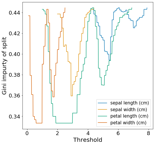
We actually observe that there are ties for the lowest weighted Gini when splitting by ‘petal length’ and by ‘petal width’.
Let’s now look at the optimal splits for each feature output by gini_best_split.
table_best_split = gini_best_split(dfIris, features, target)
| Feature | t | Gini_left | Gini_right | Gini_split |
|---|---|---|---|---|
| sepal length | 5.4 | 0.204 | 0.495 | 0.394 |
| sepal width | 2.9 | 0.481 | 0.285 | 0.360 |
| petal length | 1.9 | 0 | 0.5 | 0.333 |
| petal width | 0.6 | 0 | 0.5 | 0.333 |
As expected, we observe a tie for the lowest weighted Gini (0.333) when splitting using ‘petal length’ with threshold 1.9 and ‘petal width’ with threshold 0.6. There are two things of note here. Firstly, we know from the plot above that there are many other threshold values that would give the same weighted Gini of 0.333. The ones shown in the table are just the ones that appear first. Second, the decision classifier created by scikit-learn in Figure 1, choose to split by ‘petal length’ with threshold 2.45, which according to Figure 2 will tie for the weighted Gini score of 0.333.
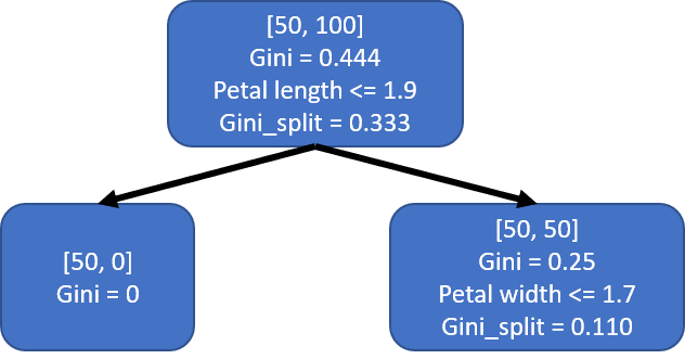
It is not clear to me how scikit-learn chooses to break ties, however, for our purpose we will choose to split by ‘petal length’ with threshold 1.9 to more closely match Figure 1. This first split creates two child nodes s1_left and s1_right, which is easily created by sub-setting dfIris.
F, t = 'petal length (cm)', 1.9
s1_left = dfIris[dfIris[F] <= t].reset_index(drop=True)
s1_right = dfIris[dfIris[F] > t].reset_index(drop=True)
This would results in a tree that looks like the one below. I labeled the nodes a little bit differently from Figure 1. The first two lines of each node show the number of each class and the Gini index of the node. The last two lines show the condition used to split the node and the weighted Gini of the split.
Second split
Since s1_left is a pure leaf node, we only need to split the s1_right node. Let’s examine the impurity of all the splits ats1_right.
s1_right_split = gini_all_splits(s1_right, features, target)

fig, ax = plt.subplots(figsize=(8, 8))
sns.lineplot(
    data=s1_right_split, x='t', y='gini_split',
    hue='Feature', palette="colorblind", markers=True)
ax.set_xlabel(xlabel='Threshold',fontsize=20)
ax.set_ylabel(ylabel='Gini impurty of split', fontsize=20)
ax.tick_params(axis='both', which='major', labelsize=18)
ax.legend(prop={'size': 15})
plt.savefig('images/iris.s1_right_split.png', bbox_inches='tight')
plt.show()
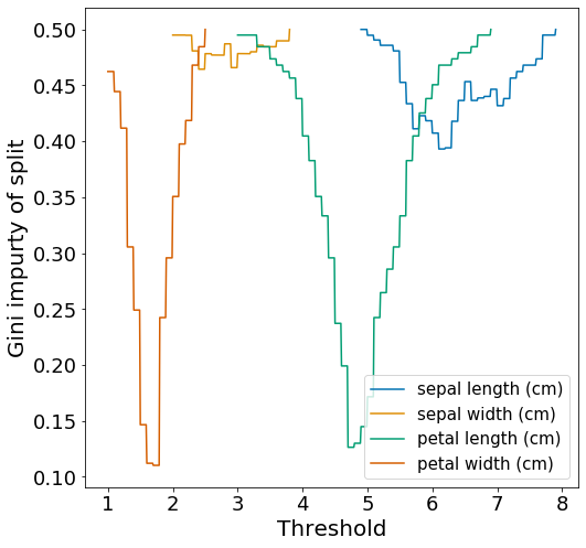
We observe that the best split is achieved by ‘petal width’. Similar to Figure 3, the ‘sepal’ traits are not very useful for splitting the dataset.
Now, let’s find the threshold and features that give the optimal split.
table_best_split = gini_best_split(s1_right, features, target)
| Feature | t | Gini_left | Gini_right | Gini_split |
|---|---|---|---|---|
| sepal length | 6.1 | 0.369 | 0.413 | 0.393 |
| sepal width | 2.4 | 0.18 | 0.496 | 0.464 |
| petal length | 4.7 | 0.043 | 0.194 | 0.126 |
| petal width | 1.7 | 0.168 | 0.043 | 0.110 |
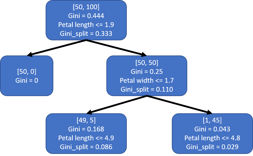
Splitting by ‘petal width’ using threshold 1.7 would be the optimal split here and results in the child nodes s2_left and s2_right.
F, t = 'petal width (cm)', 1.7
s2_left = s1_right[s1_right[F] <= t].reset_index(drop=True)
s2_right = s1_right[s1_right[F] > t].reset_index(drop=True)
The resulting decision tree would look like this:
Third split
Both s2_left and s2_right are impure, so we would need to continue splitting both of them.
For s2_left, the best split to use is ‘petal length’ with threshold 4.9.
table_best_split = gini_best_split(s2_left, features, target)

F, t = 'petal length (cm)', 4.9
s3A_left = s2_left[s2_left[F] <= t].reset_index(drop=True)
s3A_right = s2_left[s2_left[F] > t].reset_index(drop=True)
| Feature | t | Gini_left | Gini_right | Gini_split |
|---|---|---|---|---|
| sepal length | 7.0 | 0.14 | 0 | 0.137 |
| sepal width | 2.6 | 0.266 | 0.108 | 0.163 |
| petal length | 4.9 | 0.041 | 0.444 | 0.086 |
| petal width | 1.3 | 0 | 0.311 | 0.15 |
For s2_right, the best split to use is ‘petal length’ with threshold 4.8.
table_best_split = gini_best_split(s2_right, features, target)

F, t = 'petal length (cm)', 4.8
s3B_left = s2_right[s2_right[F] <= t].reset_index(drop=True)
s3B_right = s2_right[s2_right[F] > t].reset_index(drop=True)
| Feature | t | Gini_left | Gini_right | Gini_split |
|---|---|---|---|---|
| sepal length | 5.9 | 0.245 | 0 | 0.037 |
| sepal width | 3.1 | 0 | 0.133 | 0.040 |
| petal length | 4.8 | 0.444 | 0 | 0.029 |
| petal width | 1.8 | 0.153 | 0 | 0.04 |
The resulting tree after all splits:
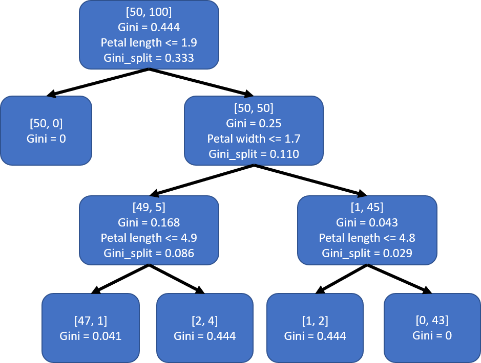
Using just a few custom functions, we have successfully reconstructed the decision tree created by scikit-learn. There are a few differences with regards to the threshold values used when splitting note but that is just because there is always a range of threshold values that would result in the exact same split.
Overall, I found this a useful exercise to get a deeper understanding of how a decision tree classifier is created. Obviously, the functions that I wrote (e.g. gini_all_splits, gini_best_split) are not the most efficient; they are actually quite slow when there are many features. There are probably more clever ways to find the local optimum split than just going through all values in a range but that is out of the scope for this post.
Construct a continuous decision tree
Just as a proof of concept, you can treat the target as a continuous variable, rather than a categorical variable, and obtain the same tree. The only difference is that instead of using the Gini index as a measure of impurity, you would use something like the mean squared error or the mean absolute error (described in Part 1).
Mean squared error (MSE):
\[H(S_{m}) = \frac{1}{N_{m}} \sum_{y} (y-\bar{y})^{2}\]Mean absolute error (MAE):
\[H(S_{m}) = \frac{1}{N_{m}} \sum_{y} |y-\tilde{y}|\]Here is the analogous set of functions to perform a step-by-step construction of a continuous decision tree using MSE as the measure of impurity. If you follow the same steps as above, you would get the exact same decision tree at the end.
def MSE(targets):
    '''
    Calculate mean squared error given list of target values
    '''
    mean_target = np.mean(targets)
    mse = sum([(x-mean_target)**2 for x in targets]) / len(targets) if len(targets)>0 else 0
    return mse

def MSE_weighted(targets_left, targets_right):
    '''
    Calculate weighted mse of split
    '''
    prop_left = len(targets_left) / (len(targets_left)+len(targets_right))
    prop_right = len(targets_right) / (len(targets_left)+len(targets_right))
    mse_split = prop_left*MSE(targets_left) + prop_right*MSE(targets_right)
    return mse_split

def mse_all_splites(data, features, target):
    '''
    Results of spliting data by each feature and a range of thresholds
    '''
    # split using each feature and each threshold
    table_split = pd.DataFrame(columns=['Feature','t','mse_left','mse_right','mse_split'])
    for F in features:
        t_min, t_max = min(data[F]), max(data[F])
        step = 0.1
        t_list = list(np.arange(t_min, t_max+step, step)) # get list of thresholds
        t_list.reverse()
        t_list = [round(x,1) for x in t_list]
        # split using each threshold and calculate gini
        for t in t_list:
            data_left = data[data[F] <= t].reset_index(drop=True)
            data_right = data[data[F] > t].reset_index(drop=True)
            mse_left = MSE(data_left[target])
            mse_right = MSE(data_right[target])
            mse_split = MSE_weighted(data_left[target], data_right[target])
            table_split.loc[len(table_split)] = [F, t, mse_left, mse_right, mse_split]
    return table_split


def mse_best_split(data, features, target):
    '''
    obtain best split for each feature
    '''
    table_split = mse_all_splites(data, features, target) # table of all splits using all features
    # get best split for each feature
    table_best_split = pd.DataFrame()
    for F in features:
        table_feature = table_split[table_split['Feature']==F].reset_index(drop=True) # subset to focal feature
        index_min_mse = table_feature.mse_split.argmin() # get index of lowest gini_split
        best_row = table_feature.iloc[index_min_mse]
        table_best_split = table_best_split.append(best_row).reset_index(drop=True)
    return table_best_split