Description of SLiM from their website:
SLiM is an evolutionary simulation framework that combines a powerful engine for population genetic simulations with the capability of modeling arbitrarily complex evolutionary scenarios. Simulations are configured via the integrated Eidos scripting language that allows interactive control over practically every aspect of the simulated evolutionary scenarios. The underlying individual-based simulation engine is highly optimized to enable modeling of entire chromosomes in large populations.
I have utilized SLiM is a couple of research projects during my PhD. Although it comes with a plethora of built-in utilities to create biologically realistic simulations, I often added custom features to suit my project needs. One of my needs were temporal fluctuations in population size (N) and selection strength (S). SLiM comes with the ability to change N and S at a specified generation(s), but I wanted to have fluctuations occur stochastically. Obviously, SLiM could not anticipate the infinite number of ways that these variable can change temporally, so I had to write my own functions.
Below if some of the SLiM scripts I developed to allow for deterministic and stochastic fluctuations in N and S.
Deterministic fluctuations of N
A simple way to have fluctuations in population size (N) is to imagine there are two environmental conditions that supports different N’s. The environment then fluctuates between these two conditions at set intervals.
Below is a simple SLiM script to have a population fluctuate between an N of 1000 and 100 every 500 generations.
initialize(){
	initializeMutationRate(1e-7); //uniform mutation rate per base per gen
	initializeMutationType("m1", 0.5, "f", 1e-4); //m1 = slightly  deleterious
	initializeGenomicElementType("g1", m1, 1); //g1 = coding site
	initializeGenomicElement(g1, 0, 99999); //Chromosome with 10000 bp
	initializeRecombinationRate(1e-8); //Assign recombination rate
}
1{
	defineConstant("N", 1000); //Set current N as 1000
	sim.addSubpop("p1", N); //Create population with size = N
}
late(){
	//Fluctuate N every 500 generations
	if(sim.generation%500 == 0){
		if(N == 1000){rm("N",T); defineConstant("N", 100);}
		else{rm("N",T); defineConstant("N", 1000);}
		p1.setSubpopulationSize(asInteger(N)); //Set population size
	}
}
10000 late(){
	sim.outputFull(); //Output full data
}
The code within initialize is pretty standard and not important here. The simulation starts at the first generation with N = 1000. Importantly, I utilize defineConstant to define N as 1000 and give it a global scope. This means that N can be called anywhere within the script, not just within 1{}.
The part within late, which runs at the end of every generation, controls the fluctuations in N. sim.generation exists by default and gives the generation number of the simulation. The modulo operation, %, within the if statement ensures that fluctuations only occur every 500 generations. The inner if statement fluctuates N by simply setting the constant N to 100 if it is currently equal 1000 or vice versa. Note that you need to use rm to remove N in order to reassign it using defineConstant. Lastly, I use setSubpopulationSize to set the population size toN.
Passing command line arguments
We can use the -d argument in the command line to pass constants used by SLiM scripts. This is essential if we want to run the script with a range of parameters.
1{
	defineConstant("N", N1); //Set current N as 1000
	sim.addSubpop("p1", N); //Create population with size = N
}
late(){
	//Fluctuate N every K generations
	if(sim.generation%K == 0){
		if(N == N1){rm("N",T); defineConstant("N", N2);}
		else{rm("N",T); defineConstant("N", N2);}
		p1.setSubpopulationSize(asInteger(N)); //Set population size
	}
}
Here, we modified the script such that the simulation fluctuates between population sizes of N1 and N2 every K generations. The command line to code to run this would simply be:
slim -d K=500 -d N1=1000 -d N2=100 MyScript.txt
Stochastic fluctuations in N
Similar to deterministic fluctuations, there are an infinite number of ways to model stochastic fluctuations in population size. Here, I will utilize a method I applied in my previous research that allows me to control the degree of temporal autocorrelation in the environments as well the frequency that each environment occurs. Again, imagine that there are two environments (E1, E2) that support two different N’s (N1, N2). I define \(\rho\) as the per generation probability that the environmental conditions remains the same; this controls for temporal autocorrelation. However, with probability 1 - \(\rho\) a “new” environment is chosen from the two. The probability of choosing E1 and E2 is defined as 1 - \(\alpha\) and \(\alpha\), respectively. Therefore, \(\alpha\) represents the expected proportion of generations the under E2.
Given this model, we can calculated the expected run length within each environment; the run length is simply the number of consecutive generations elapsed in one environment before transitioning to the other environment. The expected run length in E1 and E2 is \(((1-\rho)\alpha)^{-1}\) and \(((1-\rho)(1-\alpha))^{-1}\), respectively. You can find additional information about this model here.
Implementing this into the SLiM script only requires the use of the rbinom function to get a Bernoulli sample.
1{
	defineConstant("N", N1); //Set current N as N1
	sim.addSubpop("p1", N); //Create population with subze = N
}
late(){
	//rho is prob env stays the same
	stay = rbinom(1, 1, rho);
	//if stay==0, then randomly choose env based on alpha
	if(stay==0){
		env = rbinom(1, 1, alpha); //Choose env
		if(env==0){rm("N",T); defineConstant("N", N1);}
		else{rm("N",T); defineConstant("N", N2);}
		p1.setSubpopulationSize(asInteger(N)); //Set population size
	}
}
Each generation, we take a Bernoulli sample with probability of success equal to \(\rho\). If stay equals 1 then no change in the environment. If stay equals 0, then take another Bernoulli sample with probability of success equal to \(\alpha\) to choose the next environment. env equal to 0 and 1 means the population size changes to N1 and N2, respectively.
The command line to code to run this would simply be:
slim -d rho=0.5 -d alpha=0.5 -d N1=1000 -d N1=100 MyScript.txt
If we wanted even the environment in the first generation to be from a random sample, we can simply modify 1{} to the following:
1{
	//---Random assign initial env
	env = rbinom(1, 1, alpha); //Choose env
	if(env==0){defineConstant("N", N1);}
	else{defineConstant("N", N2);}
	sim.addSubpop("p1", N); //Create population with size = N
}
Stochastic fluctuations in S
You can also allow selection strength to fluctuate over time using the same method of simulating temporal autocorrelation. In this case, we imagine environmental conditions E1 and E2 that causes the selection coefficient to fluctuate between S1 and S2, respectively. \(\rho\) is the per generation probability that the environmental conditions remains the same. \(\alpha\) is the expected proportion of generations the under E2.
initialize(){
	initializeMutationRate(1e-7); //uniform mutation rate per base per gen
	initializeMutationType("m1", 0.5, "f", S1); //m1 = slightly  deleterious
	initializeGenomicElementType("g1", m1, 1); //g1 = coding site
	initializeGenomicElement(g1, 0, 99999); //Chromosome with 10000 bp
	initializeRecombinationRate(1e-8); //Assign recombination rate
}
1{
	defineConstant("S", S1); //set current S as S1
	sim.addSubpop("p1", N); //Create population with size = N
}
late(){
	//rho is prob env stays the same
	stay = rbinom(1, 1, rho);
	//if stay==0, then randomly choose env based on alpha
	if(stay==0){
		env = rbinom(1, 1, alpha); //Choose selection env
		if(env==0){rm("S",T); defineConstant("S", S1);}
		else{rm("S",T); defineConstant("S", S2);}

		mut = sim.mutationsOfType(m1); //get all m1 mutations
		mut.setSelectionCoeff(S); //Set selection strength for m1
	}
}
The logic here is identical to the script for stochastically fluctuating population size. To apply the change in selection coefficient, we first must get a list of all m1 mutations using sim.mutationsOfType and save it as mut. Then use setSelectionCoef to apply selection coefficient S to the mutations listed in mut.
The command line to code to run this would simply be:
slim -d rho=0.5 -d alpha=0.5 -d N=1000 -d S1=0.001 -d S2=0.0001 MyScript.txt
If we wanted even the environment in the first generation to be from a random sample, we can simply modify 1{} to the following:
1{
	//---Random assign initial env
	env = rbinom(1, 1, alpha); //Choose env
	if(env==0){defineConstant("S", S1);}
	else{defineConstant("S", S2);}
	mut = sim.mutationsOfType(m1); //get all m1 mutations
	mut.setSelectionCoeff(S); //Set selection strength for m1
}
Stochastic fluctuation model
The model for stochastic fluctuations of population size (and selection) is actually just a simple two-state Markov process.
| Symbol | Transition probability |
|---|---|
| \(p_{11}\) | \(\rho + (1-\rho) (1-\alpha)\) |
| \(p_{12}\) | \((1-\rho) \alpha\) |
| \(p_{22}\) | \(\rho + (1-\rho) \alpha\) |
| \(p_{21}\) | \((1-\rho) (1-\alpha)\) |
We can define \(T_{12}\) as the number of generations it takes to transition from N1 to N2 and \(T_{21}\) as the number of generation it takes to transition from N2 to N1; this is what I refer to as the run lengths in the sections above.
The expect value of \(T_{12}\) can be calculated following the equation for expected hitting times :
\[\begin{aligned} \overline{T_{12}} &= 1+p_{11}\overline{T_{12}} \\ \overline{T_{12}} &= (1-p_{11})^{-1} \\ \overline{T_{12}} &= (1-(\rho + (1-\rho) (1-\alpha))^{-1} \\ \overline{T_{12}} &= ((1-\rho) \alpha)^{-1} \end{aligned}\]The expect value of \(T_{21}\) can be calculated analogously:
\[\begin{aligned} \overline{T_{21}} &= 1+p_{22}\overline{T_{21}} \\ \overline{T_{21}} &= (1-p_{22})^{-1} \\ \overline{T_{21}} &= (1-(\rho + (1-\rho)\alpha)^{-1} \\ \overline{T_{21}} &= ((1-\rho)(1-\alpha))^{-1} \end{aligned}\]Visualizing the model
The mean run lengths in each environment doesn’t really tell the whole story because run lengths in this model have a very large variance. To be more precise, the run lengths are expected to be geometrically distributed, where the variance is equal to the square of the mean; it is well known that sojourn times are geometrically distributed for finite Markov models with \(p_{ii}\) > 0. This large variance in run lengths can be very impactful because it will determine how much time there is for allele frequencies to transition from one environment to the next.
To visualize the effects of \(\rho\) and \(\alpha\) on the run lengths, I simulate the model using the Python code below.
import pandas as pd
import numpy as np

def stochasticSim(rho, alpha, gen, seed):
    '''
    Simulate stochastic fluctuations following two-state Markov model
    '''
    np.random.seed(seed)
    # randomly set first environment
    ENV = np.random.binomial(1, rho)
    # run for gen generations
    lENV = [ENV]
    for x in range(gen-1):
        STAY = np.random.binomial(1, rho)
        if STAY==1:
            pass
        else:
            ENV = np.random.binomial(1, alpha)
        lENV += [ENV]
    return lENV
I will plot the first 500 generations for simulations where \(\rho = {0.5, 0.95}\) and \(\alpha = {0.5, 0.95}\).
import seaborn as sns
import matplotlib.pyplot as plt

#####-----simulate
lENV_1A = stochasticSim(0.5, 0.5, 1000, 30)
lENV_1B = stochasticSim(0.5, 0.95, 1000, 30)
lENV_2A = stochasticSim(0.95, 0.5, 1000, 30)
lENV_2B = stochasticSim(0.95, 0.95, 1000, 30)

#####-----create dataframes
lGEN = [x for x in range(1, 1000+1)]
dfEnv = pd.DataFrame({
    'GEN':lGEN+lGEN+lGEN+lGEN,
    'TYPE':[1]*1000+[2]*1000+[3]*1000+[4]*1000,
    'ENV':lENV_1A+lENV_1B+lENV_2A+lENV_2B})

#####-----plot
listI, listJ =[0,0,1,1], [0,1,0,1]
listTitle = ['\u03C1=0.5, \u03B1=0.5','\u03C1=0.5, \u03B1=0.95','\u03C1=0.95, \u03B1=0.5','\u03C1=0.95, \u03B1=0.95']

fig, ax =plt.subplots(2, 2, figsize=(15,10))
fig.subplots_adjust(hspace=0.3, wspace=0.05)
for k in range(4):
    sns.lineplot(
        data=dfEnv[dfEnv['TYPE']==(k+1)].iloc[0:500], x='GEN', y='ENV',
        markers=True, ax=ax[listI[k],listJ[k]])
    ax[listI[k],listJ[k]].set_yticks([0,1])
    ax[listI[k],listJ[k]].set_title(listTitle[k], fontsize=20, loc='left')
    if listI[k]==1:
        ax[listI[k],listJ[k]].set_xlabel(xlabel='Generation',fontsize=20)
    else:
        ax[listI[k],listJ[k]].set_xlabel(xlabel='',fontsize=20)
    if listJ[k]==1:
        ax[listI[k],listJ[k]].set_yticklabels(['', ''])
        ax[listI[k],listJ[k]].set_ylabel(ylabel='', fontsize=20)
    else:
        ax[listI[k],listJ[k]].set_yticklabels(['N1', 'N2'])
        ax[listI[k],listJ[k]].set_ylabel(ylabel='Environment', fontsize=20)
    ax[listI[k],listJ[k]].tick_params(axis='both', which='major', labelsize=18)
plt.show()
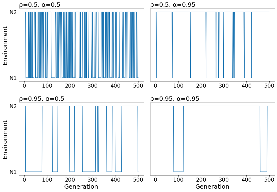
With \(\rho = 0.5, \alpha=0.5\), we observe many transitions and short run lengths in both environments. When we change the parameters to \(\rho = 0.95, \alpha=0.5\), we observe few transitions and longer run lengths because temporal autocorrelation is increased for both environments. When we adjust to \(\alpha=0.95\), we observe that population size is equal to N2 more often than N1. Since \(\alpha\) affects the expected frequency of N1 and N2, it has asymmetric effects of the temporal autocorrelation of each environment.
Now, to examine the distribution of run lengths, I use the following function which takes advantage of the groupby function:
from itertools import groupby

def calcRuns(lENV):
    '''
    Given lENV, get lengths of cosecutive runs of 0s and 1s
    '''
    lenE0, lenE1 = [], []
    for k, v in groupby(lENV):
        lV = list(v)
        if k==0:
            lenE0 += [len(lV)]
        else:
            lenE1 += [len(lV)]
    return [lenE0, lenE1]
First lets examine the distribution of run lengths with moderate temporal autocorrelation, \(\rho\), and equal frequency of each environment, \(\alpha=0.5\).
#####-----simulate
rho, alpha, gen, seed = 0.95, 0.5, 100000, 50
lENV = stochasticSim(rho, alpha, gen, seed)
lenE0, lenE1 = calcRuns(lENV)
meanE0, meanE1 = round(np.mean(lenE0),1), round(np.mean(lenE1),1)
#####-----create df
dfRuns = pd.DataFrame({'N':['N1']*len(lenE0) + ['N2']*len(lenE1),'LEN':lenE0+lenE1})
#####-----plot hitsotgram of run lengths
fig, ax = plt.subplots(figsize=(10, 10))
sns.histplot(data=dfRuns, x='LEN', hue='N', palette="colorblind")
ax.vlines(x=meanE0, ymin=0, ymax=220, color='blue', linestyle='--', alpha=0.9)
ax.vlines(x=meanE1, ymin=0, ymax=220, color='orange', linestyle='--', alpha=0.9)
ax.set_xlabel(xlabel='Run lengths',fontsize=20)
ax.set_ylabel(ylabel='Count', fontsize=20)
ax.tick_params(axis='both', which='major', labelsize=18)
ax.text(meanE0+10, 200, meanE0, fontsize=15, color='blue')
ax.text(meanE1+10, 180, meanE1, fontsize=15, color='orange')
plt.show()
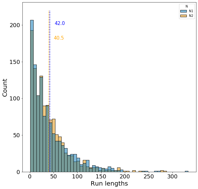
The expected run length for each environment is 40 generations under these parameters, which matches closely with the dashed lines. However, we observe the large variance in run lengths, which is expected since run lengths are geometrically distributed.
Now lets examine the distribution of run lengths with moderate temporal autocorrelation, \(\rho\), and a higher frequency of N2 environments, \(\alpha=0.95\).
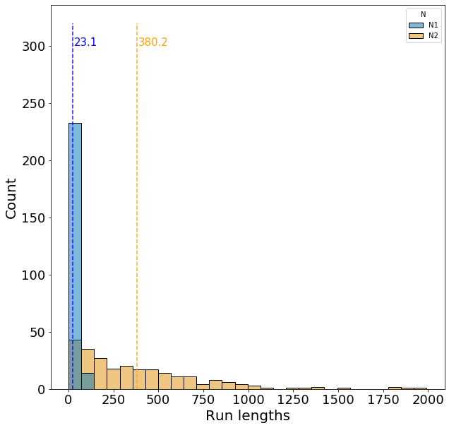
Under these parameters, the expected run length for the N1 and N2 environment is 21 and 400 generations, respectively, which matches closely with the dashed lines. Now we observe an even larger variance for run lengths in the N2 environment.